Download

1 / 35
360 likes | 489 Views
This paper explores the complex characterization of yarn hairiness, a critical property affecting textile quality. It examines methods for analyzing hairiness using Uster and Zweigle systems, discusses the limitations of traditional approaches, and introduces a bimodal analysis using Gaussian distributions. A detailed experimental methodology involving various spinning systems is presented, alongside the descriptive analysis through the HYARN program written in MATLAB. The impact of yarn hairiness on textile performance and insights into its stochastic nature are discussed, providing valuable information for textile engineering.

E N D
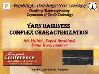
Technical University of liberec Faculty of Textile engineering Department of Textile Technology Yarn HAIRINESS COMPLEX CHARACTERIZATION Jiří Militký, Sayed Ibrahim& Dana Kremenakova 7-8 May 2009, Lahore, Pakistan
Introduction • Hairiness is considered as sum of the fibre ends and loops standing out from the main compact yarn body • The most popular instrument is the Uster hairiness system, which characterizes the hairiness by H value, and is defined as the total length of all hairs within one centimetre of yarn. • The system introduced by Zweigle, counts the number of hairs of defined lengths. The S3 gives the number of hairs of 3mm and longer. • The information obtained from both systems are limited, and the available methods either compress the data into a single vale H or S3, convert the entire data set into a spectrogram deleting the important spatial information. • Some laboratory systems dealing with image processing, decomposing the hairiness function into two exponential functions (Neckar,s Model), time consuming, dealing with very short lengths. Uster Hairiness Uster tester Zweigle Hairiness
Principle of Different Spinning Systems Ring-Compact Spinning Principle of Siro OE Spinning Vortex Spinning
Outline • Investigation the possibility of approximation yarn hairiness distribution as a mixture of two Gaussian distributions. • Techniques for basic assumptions about hairiness variation curve from USTER Tester • Solution of inverse problem i.e. specification of the characteristics of the underlying stochastic process. • Description of HYARN program for complex analysis of hairiness data
1st Part bimodality USTER hairiness diagram The signal from hairiness measurement between distances di is equal to the overall length of fibers protruded from the body of yarn on the length = 1 cm. This signal is expressed in the form of the hairiness diagram (HD). The raw data from Uster tester 4 were extracted and converted to individual readings corresponding to yarn hairiness, i.e. the mean value of total hair length per unit length (centimeter).
Experimental Part andMethod of Evaluation More than 75 cotton different yarns (14.5-30 tex) of different counts were spun on different spinning systems, namely ring, compact, Siro-spun, Open-end spinning, plied yarns, and vortex yarn of count 20 tex, spun from viscose fibers. All of these yarns were tested against yarn hairiness. Hair Diagram Histogram (83 columns) Normal Dist. fit OE Yarn Gaussian curve fit (20 columns) Smooth curve fit
Basics of Probability Density Function Optimising Number of Pins • The area of a column in a histogram represents a piecewise constant estimator of sample probability density. Its height is estimated by: • Where is the number of sample • elements in this interval • and is the length • of this interval. • Number of classes • For all samples is N= 18458 and M=125 and h = 0.133
Kernel Density Function The Kernel type nonparametric (free function) of sample probability density function Kernel function : bi-quadratic symmetric around zero, has the same properties as PDF Optimal bandwidth : h 1.Based on the assumptions of near normality 2.Adaptive smoothing 3. Exploratory (local hj) requirement of equal probability in all classes h = 0.1278
Bi-modal distributionTwo Gaussian Distribution The bi-modal distribution can be approximated by two Gaussian distributions: Where , are proportions of shorter and longer hair distribution respectively, , are the means and , are the standard deviations. H-yarn Program written in Matlab code, using the least square method is used for estimating these parameters. these parameters.
Analysis of Results Significance of Bi-Modality Distribution Bimodality Parametric Tests: • Mixture of distributions estimation and likelihood ratio test • Test of significant distance between modes (Separation) Bimodality Nonparametric Tests: • kernel density (Silverman test) • CDF (DIP, Kolmogorov tests) • Rankit plot
Mixture of two Gaussian Distributions Mixture of two distributions does not necessarily result always in a bimodal distribution.
Dip Test I Dip test statistics: It is the largest vertical difference between the empirical cumulative distribution FE and the Uniform distribution FU Points A and B are modes, shaded areas C,D are bumps, area E is the dip and F is a shoulder point
Analysis of Results IIMixture of Gauss distributions Probabilitydensity function (PDF) f (x), Cumulative Distribution Function (CDF) F (x), and Empirical CDF (ECDF) Fn(x) Uni-modal CDF: is convex in (−∞, m), and concave in [m, ∞) Bimodal CDF: one bump Let Gp = arg min supx |Fn(x) − G(x)|, Where G(x) is a unimode CDF. Dip Statistic: d = supx |Fn(x) − Gp(x)| Dip Statistic (for n= 18500): 0.0102 Critical value (n = 1000): 0.017 Critical value (n = 2000): 0.0112
Analysis of Results IIILikelihood ratio test The single normal distribution model (μ,σ), the likelihood function is: Where the data set contains n observations. The mixture of two normal distributions, assumes that each data point belongs to one of two sub-population. The likelihood of this function is given as: The likelihood ratio can be calculated from Lu (uni-modal) and Lb (bi-modal) asfollows:
Analysis of Results IV Significance of difference of means • Two sample t test of equality of means • T1 equal variances • T2 different variances
Analysis of Results VI PDF and CDF Kernel density estimator: Adaptive Kernel Density Estimator for univariate data. (choice of band width h determines the amount of smoothing. If a long tailed distribution, fixed band width suffer from constant width across the entire sample (noise). For very small band width an over smoothing may occur . MATLAB AKDEST 1D- evaluates the univ-ariate Adaptive Kernel Density Estimate with kernel.
Basic definitions of Time Series • Since, the yarn hairiness is measured at equal-distance (equal time interval), the data obtained could be analyzed on the base of time series. • A time series is a sequence of observations taken sequentially in time. The nature of the dependence among observations of a time series is of considerable practical interest. • First of all, one should investigate the stationarity of the system. • Stationary model assumes that the process remains in equilibrium about a constant mean level. The random process is strictly stationary if all statistical characteristics and distributions are independent on ensemble location. • Many tests such as nonparametric test, run test, variability (difference test), cumulative periodogram construction are provided to explore the stationarity of the process. The H-yarn is capable of estimating all of these parameters.
Basic assumptions I Let the Hairiness relative deviation y(i) is a series “spatial” realization of random process y = y(di). For analysis of this series it is necessary to know if some basic assumptions about behavior of underlying random process can be accepted stationarity ergodicity independency In fact the realizations of random process are yj(i), where index j correspond to individual realizations and index icorresponds to the distance di. In the case of ensemble,samples, there are values yj(i) fori = const. and j = 1..M at disposal. In majority of applications the ensemble samples are not available and statistical analysis is based on the one spatial realization yj(i) for j = 1 and i = 1..N. realization yj(i) forj = const. ,j = 1..N ensemble Real yarn yj(i) for i = const. ,j = 1..M For creation of data distribution and computation of moments, additional assumptions are necessary
Stationarity The random process is strictly stationary if all statistical characteristics and distributions are independent on ensemble location, i.e. the mean and variance, do not change over time or position. The wide sense stationarity of g-th order implies independence of first g moments on ensemble location. The second order stationarity implies that: mean value E(y(i)) = E(y) is constant (not dependent on the location di). VarianceD(y(i)) = D(y) is constant (not dependent on the location di). autocovariance, autocorrelation and variogram, which are functions of di and dj are not dependent on the locations but on the lag only E(y)=0
Ergodicity Ergodic process- the “ensemble” mean can be replaced by the average across the distance (from one spatial realization) Autocorrelation R(h) =0 for all sufficiently high h Ergodicity is very important, as the statistical characteristics can be calculated from one single series y(i) instead of ensembles which frequently are difficult to be obtained.
Inverse problem Inverse problem - given a series y(i), how to discover the characteristics of the underlying process. Three approaches are mainly applied: • first based on random stationary processes, • second based on the self affine processes with multi-scale nature, • third based on the theory of chaotic dynamics. In reality the multi-periodic components are often mixed with random noise.
Distribution check In most methods for data processing based on stochastic models, normal distribution is assumed. If the distribution is proved to be non-normal there are three possibilities: • the process is linear but non-Gaussian; • the process has linear dynamics, but the data are result of non-linear ”static” transformation • the process has non-linear dynamics. Real yarn The histograms for four sub samples (division of data of 400 meter yarn into 100 meter pieces).
Pseudo ensemble analysis It is suitable to construct the histograms for the e.g. four quarters of data separately and inspect non-normality or asymmetry of distribution. The statistical characteristics (mean and variances) of these sub series can support wide sense stationarity assumption The t-test statistics for comparison of two most distant means The F ratio statistics for comparison of two most distant variances
Stationarity graphs I Zero order variability diagramplot of y(i+1) on y(i). In the case of independence the random cloud of points appears on this graph. Autocorrelation of first order is indicated by linear trend. First order variability diagram is constructed taking the first differences d1(i) = y(i) – y(i-1) as new data set. The second order variability diagram is then dependence of d1(i+1) on d1(i). This diagram “correlates” three successive elements of series y(i). Second order variability diagramfor the second differences d2(i) =d1(i) –d1(i-1) Third order variability diagramfor the third order differences d3(i)=d2(i) –d2(i-1). As the order of variability diagram increases the domain of correlations increases as well.
Stationarity graphs II For characterization of independence hypothesis against periodicity alternative the cumulative periodogramC(fi) can be constructed. For white noise series (independent identical distribution i.i.d normally distributed data), the plot of C(fi) against fiwould be scattered about a straight line joining the points (0,0) and (0.5,1). Periodicities would tend to produce a series of neighboring values of I(fi) which were large. The result of periodicities therefore bumps on the expected line. The limit lines for 95 % confidence interval of C(fi) are drawn at distances
y x Spatial correlations Autocovariance function Second equality is valid for centered data E(y) = 0 and wide sense stationarity (autocovariance is dependent on the lag h and not on the positions i). For lag h = 0 the variance results s2 = v = c(0). Autocorrelation function y(i) i =0..N-1
AutocorrelationR(1) Simply the Autocorrelation function is a comparison of a signal with itself as a function of time shift. Autocorrelation coefficient of first order R(1) can be evaluated as Roughly, if R(1) is in interval no autocorrelation of first order is identified.
Frequency domain The Fast Fourier Transformation is used to transform from time domain to frequency domain and back again is based on Fourier transform and its inverse. There are many types of spectrum analysis, PSD, Amplitude spectrum, Auto regressive frequency spectrum, moving average frequency spectrum, ARMA freq. Spectrum and many other types are included in Hyarn program.
Fractal DimensionHurst Exponent The cumulative of white Identically Distribution noise is known as Brownian motion or a random walk. The Hurst exponent is a good estimator for measuring the fractal dimension. The Hurst equation is given as . The parameter H is the Hurst exponent. In measurement of surface profile (R(h)), the data are available through one dimensional line transect surface. The fractal dimension can be measured by 2-H. In this case the cumulative of white noise will be 1.5. More useful is expressing the fractal dimension by 1/H using probability space rather than geometrical space. Fractal dimension D is then number between 1 (for smooth curve) and 2. One of best methods for evaluation of or H is based on the power spectral density For small Fourierfrequencies is often evaluated from empirical representation of the log of power spectral density versus log frequency.
Summary of results of ACF, Power Spectrum and Hurst Exponent Samples from H-Yarn program. Autocorrelation, Spectrum, Hurst graphs.
Conclusions • The yarn hairiness distribution can be fitted to a bimodal model distribution. • described by two mixed Gaussian distributions. • The portion, mean and the standard deviation of each component leads to deeper understanding and evaluation of hairiness. • This method is quick compared to image analysis system, • The Hyarn system is a powerful program for evaluation and analysis of yarn hairiness as a dynamic process, in both time and frequency domain. • H-yarn program is capable of estimating the short and long term dependency. • Hairiness of Vortex yarn is lowest followed by compact yarns. • Siro spun yarns have less values compared to ring and plied and open-end yarns. This is mainly observed due to the short component and the portion of hairs. • The highest values of hairiness belong to plied yarns, since they pass more operations (doubling and twisting).