Download
1 / 32
320 likes | 529 Views
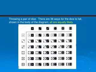
Throwing a pair of dice. There are 36 ways for the dice to fall, shown in the body of the diagram; all are equally likely . Example . A pair of dice are thrown. What is the chance of getting a total of 4 spots? Solution . Look at the figure. There are 3 ways to get a total of four spots:.

E N D
Throwing a pair of dice. There are 36 ways for the dice to fall, shown in the body of the diagram; all are equally likely.
Example. A pair of dice are thrown. What is the chance of getting a total of 4 spots? Solution. Look at the figure. There are 3 ways to get a total of four spots: The chance is 3 in 36. That is the answer.
Sample Space • Probability theory is used as a model for situations for which the outcomes occur randomly. Generically, such situations are called “experiments,” and the set of all possible outcomes is the sample space corresponding to an experiment. The sample space is denoted by , and a generic element of is denoted by . The following are some examples.
Example • A driver passes through a sequence of three intersections with traffic lights. At each light, the driver either stops, s, or continues,c. The sample space is the set of all possible outcomes: = {ccc, ccs, css, csc, sss, ssc, scc, scs} Where csc, for example, denotes the outcome that the commuter continues through the first light, stops at the second light, and continues through the third light.
Example • The number of jobs in a print queue of a computer may be modeled as random. Here the sample space can be taken as = {0, 1, 2, 3 …} that is, all the nonnegative integers. In practice, there is probably an upper limit, N, on how large the print queue can be, so instead the sample space might be defined as = {0, 1, 2, …, N}
Example • Earthquakes exhibit very erratic behavior, which is sometimes modeled as random. For example, the length of time between successive earthquakes in a particular region that are greater in magnitude than a given threshold may be regarded as an experiment. Here is the set of all nonnegative real numbers. = { t | t ≥ 0 }
We are often interested in particular subsets of , which in probability language are called events. In the first example the event that the driver stops at the first light is the subset of denoted by • A = { sss, ssc, scc, scs } • (Events, or subsets, are usually denoted by italic uppercase letters.) In the second example, the event that there are fewer than five jobs in the print queue can be denoted by • A = { 0, 1, 2, 3, 4 }
The algebra of set theory carries over directly into probability theory. The union of two events, A and B, is the event C that either A occurs or B occurs or both occur: C = A B. For example, if A is the event that the driver stops at the first light (listed above) and if B is the event that he or she stops at the third light, B = { sss, scs, ccs, css } then C is the event that the driver stops at the first light or stops at the third light and consists of the outcomes that are in A or B or in both: C = { sss, ssc, scc, scs, ccs, css }
The intersection of two events, C = A B, is the event that both A and B occur. If A and B are listed above, then C is the event that the driver stops at the first light and stops at the third light and thus consists of those outcomes that are common to both A and B: C = { sss, scs } The complement of an event, Ac , is the event that A does not occur and thus consists of all those elements in the sample space that are not in A. The complement of the event that the driver stops at the first light is the event that he or she continues at the first light Ac= { ccc, ccs, css, csc } You may recall the empty set is usually denoted by . The empty set is the set with no elements; it is the event with no outcomes. An event of probability 0 may or may not be empty. If A is the event that the driver stops at the first light and C is the event of continuing through all three lights, C = { ccc }, then A and C have no outcomes in common, and we can write A C =
In such cases, A and C are said to be disjoint. Venn diagrams, such as those below, are often a useful tool for visualizing set operations. Figure. Venn diagrams of A B and A B.
The following are some laws of set theory. Cummutative Laws: A B = B A A B = B A Associative Laws: (A B) C = A (B C) (A B) C = A (B C) Distributive Laws: (A B) C = (A C) (B C) (A B) C = (A C) (B C) Of these, the distributive laws are the least intuitive, and you may find it instructive to illustrate them with Venn diagrams.
Probability Measures Our course is not about the foundations of probability, so we will give this important topic only slight mention for now. However, the problem is that we will repeatedly be making statements that have probabilities as their “backbones.” We will speak of “the probability of disease given underlying conditions or parameters,” alternatively of “the probability of data as discrepant or more so with a null hypothesis than those that were observed.” It is difficult if not impossible to ignore the issue of what is meant by these statements. In particular, there will always be the question as to whom or what any results or statements made apply. Fortunately, in many instances while different notions of probability cannot possibly give exactly identical answers, the “answers” are nearly the same if each is applied with suitable care. Before moving on to much too brief definitions, we note that often the operational justifications of statements about probability we will make depend upon a frequentistic definition, even though the intuitive approaches we keep in the backs of our minds are rather subjective.
Frequentistic approach. For repeated events, probability can be estimated by the “long run” relative frequency of an event out of a set of many trials. If an event occurs m times in n trials, then the relative frequency m/n provides an “unbiased” estimate of the probability of the event. In the limit, as the number of trials n increases without bound, the relative frequency converges to the “true” probability of the event (“Law of Large Numbers”). This interpretation involving repeated trials is known as the “frequentist” approach to probability.
Non-frequentist subjective approach. • The frequentist approach has a number of disadvantages. First, it cannot be used to provide probability statements for events that occur once or only rarely (for example, change in a particular pattern of weather). Second, the frequentist estimates are based entirely on the sample and so cannot take into account any priori belief (common or other sense) about the probability. Think of flipping a coin 25 times and asking yourself based on the results whether the coin is “fair”. The subjective probability of an event A can be defined as the price you would pay for a fair bet on the event divided by the amount you would win if the event happens. Fair means that neither you nor the bookmaker would be expected to make any profit. To make a fair bet, prior information must be taken into account. Well-meaning people faced with the same data can have very different opinions. • Laplace’s law of succession. • The Reverend Thomas Bayes.
A probability measure on is a function P from subsets of to the real numbers that satisfies the following axions: • P ( ) = 1 • If A , then P(A) ≥ 0. • If A1 and A2 are disjoint, then • P(A1 A2) = P(A1) + P(A2) • Most generally, ifA1, A2, …, An, … are mutually disjoint, then • P( Ai ) = P (Ai) 1 i =1
The first two axioms are rather obvious. Since consists of all possible outcomes P() = 1. The second axiom simply states that a probability is nonnegative. The third axiom states that if A and B are disjoint – that is, have no outcomes in common – then P(A B) = P(A) + P(B), and also that this property extends to limits. For example, the probability that the print queue contains either one or three jobs is equal to the probability that it contains one plus the probability that it contains three. The following properties of probability measures are consequences of the axioms. PROPERTY A. P (Ac) = 1 – P(A). This property follows since A and Ac are disjoint with A Ac = and thus, by the first and third axioms, P(A) + P(Ac)= 1. In words, this porperty says that the probability that an event does not occur equals one minus the probability that it does occur.
Property B. P () = 0. This property follows from Property A since = c . In words, this says that the probability that there is no outcome at all is zero. Property C. If A B, then P(A) P(B). This property follows since B can be expressed as the union of two disjoint sets: B = A (B Ac ) Then, from the third axiom, P (B) = P (A) + P ( B Ac) And thus P (A) = P (B) – P (B Ac) P (B) This property states that if B occurs whenever A occurs, then P(A) P(B). For example, if whenever it rains (A) it is cloudy (B), then the probability that it rains is less than or equal to the probability that it is cloudy.
Property D. (Addition Law) P (A B) = P (A) + P (B) – P (A B). To see this, we decompose A B into three disjoint subsets, as shown in the following figure. C = A Bc D = A B E = Ac B We then have, from the third axiom, P (A B) = P (C) + P (D) + P (D) + P (E)
Also, A = C D, and C and D are disjoint; so P(A) = P(C) + P (D). Similarly, P(B) + P(D) + P(E). Putting these results together, we see that P (A) + P (B) = P (C) + P(E) + 2 P (D) = P (A B ) + P (D) or P (A B ) = P (A) + P (D) – P (D) This property is easy to see from the Venn diagram. If P (A) and P (B) are added together, P (A B) is counted twice.
EXAMPLE. Suppose that a fair coin is thrown twice. Let A denote the event of heads on the first toss and B the event of heads on the second toss. The sample space is = { hh, ht, th, tt } We assume that each elementary outcome in is equally likely and has probability ¼ . C = A B is the event that heads comes up on the first toss or on the second toss. Clearly, P(C) P(A) + P(B) = 1. Rather, since A B is the event that heads comes up on the first toss and on the second toss, P (C) = P (A) + P (B) – P (A B) = .5 + .5 - .25 = .75
Computing Probabilities: Counting Methods Probabilities are especially easy to compute for finite sample spaces. Suppose that = { 1, 2, …, N } and that P ( i ) = pi. To find the probability of an event A, we simply add the probabilities of the i that constitute A. EXAMPLE. Suppose that a fair coin is thrown twice and the sequence of heads and tails is recorded. The sample space is = { hh, ht, th, tt } As in the previous example, we assume that each outcome in has probability .25. Let A denote the event that at least one head is thrown. The A = { hh, ht, th }, and P(A) = .75.
This is a simple example of a fairly common situation. The elements of all have equal probability; so if there are N elements in , each of them has probability 1/N. If A can occur in any of n mutually exclusive ways, then P(A) = n/N, or P(A) = -------------------------------------------------- Note that this formula holds only if all the outcomes are equally likely. In Example A, if only the number of heads were recorded, then would be { 0, 1, 2}. These outcomes are not equally likely, and P (A) is not 2/3. The preceding example is a very simple case. To compute probabilities for more complex situations, we must develop systematic ways of counting outcomes. number of ways A can occur total number of outcomes
The Multiplication Principle The following is a statement of the very useful multiplication principle. MULTIPLICATION PRINCIPLE. If one experiment has m outcomes and another experiment has n outcomes, then there are mn possible outcomes for the two experiments. EXAMPLE. A DNA molecule is a sequence of four types of nucleotides, denoted by A, G, C, and T. The module can be millions of units long and can thus encode an enormous amount of information. For example, for a molecule 1 million units long, there are 410different possible sequences. This is a staggeringly large number having nearly a million digits. An amino acid is coded for by a sequence of three nucleotides; there are 43 = 64 different codes, but there are only 20 amino acids since some of them can be coded for in several ways. A protein molecule is composed of as many as hundreds of amino acid units and thus there are an incredibly large number of possible proteins. For example, there are 20100different sequences of 100 amino acids. 6
EXAMPLE. (Birthday Problem) Suppose that a room contains n people. What is the probability that at least two of them have a common birthday? This is a famous problem with a counterintuitive answer. Assume that every day of the year is equally likely to be a birthday, disregard leap years, and denote by A the event that there are at least two people with a common birthday. As is sometimes the case, it is easier to find P(Ac) than to find P(A). This is because A can happen in many ways, whereas Ac is much simpler. There are 365n possible outcomes, and Ac can happen in 365 x 364 x (365 – n + 1) ways. Thus, P (Ac) = -------------------------------------------- 365 x 364 x … x (365 –n + 1) 365n
The following table exhibits the latter probabilities for various values of n: n P(A) ------------ 4 .016 16 .284 23 .507 32 .753 40 .891 56 .988 From the table, we see that if there are only 23 people, the probability of at least one match exceeds .5.
The PARADOX OF THE CHEVALIER DE MÉRÉ • In the seventeenth century, French gamblers used to bet on the event that with 4 rolls of a die, at least one ace would turn up; an ace is . In another game, they bet on the event that with 24 rolls of a pair of dice, at least one double-ace would turn up: a double-ace is a pair of dice which show . • The Chevalier de Méré, a French nobleman of the period, thought the two events were equally likely. He reasoned this way about the first game: • In one roll of a die, I have 1/6 of a chance to get an ace. • So in 4 rolls, I have 4 x 1/6 = 2/3 of a chance to get at least • one ace.
His reasoning for the second game was similar: • In one roll of a pair of dice, I have 1/36 of a chance to get a double-ace. • So in 24 rolls, I must have 24 x 1/36 = 2/3 of a chance to get at least • one double-ace. • By this argument, both chances were the same, namely 2/3. But experience showed the first event to be a bit more likely than the second. This contradiction became known as the Paradox of the Chevalier de Méré. • De Méré asked the philosopher Blaise Pascal about the problem, and Pascal solved it with the help of his friend, Pierre de Fermat. Fermat was a judge and a member of parliament, who is remembered today for the mathematical research he did after hours. Fermat saw that de Méré was adding chances for events that were not mutually exclusive. In fact, using de Méré’s argument a little further, it shows the chance of getting an ace in 6 rolls of a die to be 6/6, or 100%. Something had to be wrong.
The question is how to calculate the chances correctly. Pascal and Fermat solved this problem, with a typically indirect piece of mathematical reasoning – the kind that always leaves non-mathematicians feeling a bit cheated. Of course, a direct attack could easily bog down: with 4 rolls of a die, there are 64 = 1,296 outcomes to worry about; with 24 rolls of a pair of dice, there are 3624 2.2 x 1037 outcomes. The conversation between Pascal and Fermat is lost to history, but here is a reconstruction.
Pascal. Let’s look at the first game first. Fermat. Bon. The chance of winning is hard to compute, so let’s work out the chance of the opposite event – losing. Then chance of winning = 100% -- chance of losing. Pascal. D’accord. The gambler loses when none of the four rolls shows an ace. But how do you work out the chances? Fermat. It does look complicated. Let’s start with one roll. What’s the chance that the first roll doesn’t show an ace? Pascal. It has to show something from 2 through 6, so the chance is 5/6. Fermat. C’est ça. Now, what’s the chance that the first two rolls don’t show aces?
Pascal. We can use the multiplication rule. The chance that the first roll doesn’t give an ace and the second doesn’t give an ace equals 5/6 x 5/6 = (5/6)2. After all, the rolls are independent, n’est-ce pas? Fermat. What about 3 rolls? Pascal. It looks like 5/6 x 5/6 x 5/6 = (5/6)3. Fermat. Oui. Now what about 4 rolls? Pascal. Must be (5/6)4. Fermat. Yes, and that’s about 0.482, or 48.2%.
Pascal. So there is a 48.2% chance of losing. Now chance of winning = 100% - chance of losing = 100% - 48.2% = 51.8%. Fermat. That settles the first game. The chance of winning is a little over 50%. Now what about the second? Pascal. Well, in one roll of a pair of dice, there is 1 chance in 36 of getting a double-ace, and 35 chances in 36 of not getting a double-ace. By the multiplication rule, in 24 rolls of a pair of dice the chance of getting no double-aces must be (35/36)24 .
Fermat. Eh bien, that’s about 50.9%. So we have the chance of losing. Now chance of winning = 100% - chance of losing = 100% - 50.9% = 49.1%. Pascal. Yes, and that’s a bit less than 50%. Voilà. That’s why you win the second game a bit less frequently than the first. But you have to roll a lot of dice to see the difference. This example illustrates one strategy for working out chances: if the chance of an event is hard to find, try to find the chance of the opposite event; then subtract from 100%. This is useful when the chance of the opposite event is easier to compute.