Chapter 4 Classification
Chapter 4 Classification. Classification: Definition. Given a collection of records ( training set ) Each record contains a set of attributes , one of the attributes is the class . Find a model for class attribute as a function of the values of other attributes.


Chapter 4 Classification
E N D
Presentation Transcript
Chapter 4 Classification
Classification: Definition • Given a collection of records (training set ) • Each record contains a set of attributes, one of the attributes is the class. • Find a model for class attribute as a function of the values of other attributes. • Goal: previously unseen records should be assigned a class as accurately as possible. • A test set is used to determine the accuracy of the model. Usually, the given data set is divided into training and test sets, with training set used to build the model and test set used to validate it.
Examples of Classification Task • Predicting tumor cells as benign or malignant • Classifying credit card transactions as legitimate or fraudulent • Classifying secondary structures of protein as alpha-helix, beta-sheet, or random coil • Categorizing news stories as finance, weather, entertainment, sports, etc
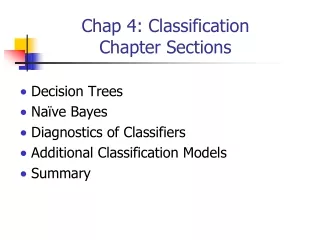
Classification Techniques • Decision Tree based Methods • Rule-based Methods
categorical categorical continuous class Example of a Decision Tree Splitting Attributes Refund Yes No NO MarSt Married Single, Divorced TaxInc NO < 80K > 80K YES NO Model: Decision Tree Training Data
NO Another Example of Decision Tree categorical categorical continuous class Single, Divorced MarSt Married NO Refund No Yes TaxInc < 80K > 80K YES NO There could be more than one tree that fits the same data!
Decision Tree Classification Task Decision Tree
Refund Yes No NO MarSt Married Single, Divorced TaxInc NO < 80K > 80K YES NO Apply Model to Test Data Test Data Start from the root of tree.
Refund Yes No NO MarSt Married Single, Divorced TaxInc NO < 80K > 80K YES NO Apply Model to Test Data Test Data
Apply Model to Test Data Test Data Refund Yes No NO MarSt Married Single, Divorced TaxInc NO < 80K > 80K YES NO
Apply Model to Test Data Test Data Refund Yes No NO MarSt Married Single, Divorced TaxInc NO < 80K > 80K YES NO
Apply Model to Test Data Test Data Refund Yes No NO MarSt Married Single, Divorced TaxInc NO < 80K > 80K YES NO
Apply Model to Test Data Test Data Refund Yes No Assign Cheat to “No” NO MarSt Married Single, Divorced TaxInc NO < 80K > 80K YES NO
Decision Tree Classification Task Decision Tree
Decision Tree Induction • Many Algorithms: • Hunt’s Algorithm (one of the earliest) • CART • ID3, C4.5 • SLIQ,SPRINT
General Structure of Hunt’s Algorithm • Let Dt be the set of training records that reach a node t • General Procedure: • If Dt contains records that belong the same class yt, then t is a leaf node labeled as yt • If Dt is an empty set, then t is a leaf node labeled by the default class, yd • If Dt contains records that belong to more than one class, use an attribute test to split the data into smaller subsets. Recursively apply the procedure to each subset. Dt ?
Refund Refund Yes No Yes No Don’t Cheat Marital Status Don’t Cheat Marital Status Single, Divorced Refund Married Married Single, Divorced Yes No Don’t Cheat Taxable Income Cheat Don’t Cheat Don’t Cheat Don’t Cheat < 80K >= 80K Don’t Cheat Cheat Hunt’s Algorithm Don’t Cheat
Tree Induction • Greedy strategy. • Split the records based on an attribute test that optimizes certain criterion. • Issues • Determine how to split the records • How to specify the attribute test condition? • How to determine the best split? • Determine when to stop splitting
Tree Induction • Greedy strategy. • Split the records based on an attribute test that optimizes certain criterion. • Issues • Determine how to split the records • How to specify the attribute test condition? • How to determine the best split? • Determine when to stop splitting
How to Specify Test Condition? • Depends on attribute types • Nominal • Ordinal • Continuous • Depends on number of ways to split • 2-way split • Multi-way split
CarType Family Luxury Sports CarType CarType {Sports, Luxury} {Family, Luxury} {Family} {Sports} Splitting Based on Nominal Attributes • Multi-way split: Use as many partitions as distinct values. • Binary split: Divides values into two subsets. Need to find optimal partitioning. OR
Size Small Large Medium Size Size Size {Small, Medium} {Small, Large} {Medium, Large} {Medium} {Large} {Small} Splitting Based on Ordinal Attributes • Multi-way split: Use as many partitions as distinct values. • Binary split:Divides values into two subsets. Need to find optimal partitioning. • What about this split? OR
Splitting Based on Continuous Attributes • Different ways of handling • Discretization to form an ordinal categorical attribute • Static – discretize once at the beginning • Dynamic – ranges can be found by equal interval bucketing, equal frequency bucketing(percentiles), or clustering. • Binary Decision: (A < v) or (A v) • consider all possible splits and finds the best cut • can be more compute intensive
Tree Induction • Greedy strategy. • Split the records based on an attribute test that optimizes certain criterion. • Issues • Determine how to split the records • How to specify the attribute test condition? • How to determine the best split? • Determine when to stop splitting
How to determine the Best Split Before Splitting: 10 records of class 0, 10 records of class 1 Which test condition is the best?
How to determine the Best Split • Greedy approach: • Nodes with homogeneous class distribution are preferred • Need a measure of node impurity: Non-homogeneous, High degree of impurity Homogeneous, Low degree of impurity
Measures of Node Impurity • Gini Index • Entropy • Misclassification error
M0 M2 M3 M4 M1 M12 M34 How to Find the Best Split Before Splitting: A? B? Yes No Yes No Node N1 Node N2 Node N3 Node N4 Gain = M0 – M12 vs M0 – M34
Measure of Impurity: GINI • Gini Index for a given node t : (NOTE: p( j | t) is the relative frequency of class j at node t). • Maximum (1 - 1/nc) when records are equally distributed among all classes, implying least interesting information • Minimum (0.0) when all records belong to one class, implying most interesting information
Examples for computing GINI P(C1) = 0/6 = 0 P(C2) = 6/6 = 1 Gini = 1 – P(C1)2 – P(C2)2 = 1 – 0 – 1 = 0 P(C1) = 1/6 P(C2) = 5/6 Gini = 1 – (1/6)2 – (5/6)2 = 0.278 P(C1) = 2/6 P(C2) = 4/6 Gini = 1 – (2/6)2 – (4/6)2 = 0.444
Splitting Based on GINI • Used in CART, SLIQ, SPRINT. • When a node p is split into k partitions (children), the quality of split is computed as, where, ni = number of records at child i, n = number of records at node p.
Binary Attributes: Computing GINI Index • Splits into two partitions • Effect of Weighing partitions: • Larger and Purer Partitions are sought for. B? Yes No Node N1 Node N2 Gini(N1) = 1 – (5/6)2 – (2/6)2= 0.194 Gini(N2) = 1 – (1/6)2 – (4/6)2= 0.528 Gini(Children) = 7/12 * 0.194 + 5/12 * 0.528= 0.333
Categorical Attributes: Computing Gini Index • For each distinct value, gather counts for each class in the dataset • Use the count matrix to make decisions Multi-way split Two-way split (find best partition of values)
Continuous Attributes: Computing Gini Index • Use Binary Decisions based on one value • Several Choices for the splitting value • Number of possible splitting values = Number of distinct values • Each splitting value has a count matrix associated with it • Class counts in each of the partitions, A < v and A v • Simple method to choose best v • For each v, scan the database to gather count matrix and compute its Gini index • Computationally Inefficient! Repetition of work.
Sorted Values Split Positions Continuous Attributes: Computing Gini Index... • For efficient computation: for each attribute, • Sort the attribute on values • Linearly scan these values, each time updating the count matrix and computing gini index • Choose the split position that has the least gini index
Notes on Overfitting • Overfitting results in decision trees that are more complex than necessary • Training error no longer provides a good estimate of how well the tree will perform on previously unseen records • Need new ways for estimating errors
Causes of Overfitting • Noise or errors in data • Lack of Representative samples • Inherent in multiple comparison procedures!
Estimating Generalization Errors • Re-substitution errors:error on training ( e(t) ) • Generalization errors: error on testing ( e’(t)) • Methods for estimating generalization errors: • Optimistic approach: e’(t) = e(t) • Pessimistic approach: • For each leaf node: e’(t) = (e(t)+0.5) • Total errors: e’(T) = e(T) + N 0.5 (N: number of leaf nodes) • For a tree with 30 leaf nodes and 10 errors on training (out of 1000 instances): Training error = 10/1000 = 1% Generalization error = (10 + 300.5)/1000 = 2.5% • Reduced error pruning (REP): • uses validation data set to estimate generalization error
Occam’s Razor • Given two models of similar generalization errors, one should prefer the simpler model over the more complex model • For complex models, there is a greater chance that it was fitted accidentally by errors in data • Therefore, one should include model complexity when evaluating a model
Minimum Description Length (MDL) • Cost(Model,Data) = Cost(Data|Model) + Cost(Model) • Cost is the number of bits needed for encoding. • Search for the least costly model. • Cost(Data|Model) encodes the misclassification errors. • Cost(Model) uses node encoding (number of children) plus splitting condition encoding.
How to Address Overfitting • Pre-Pruning (Early Stopping Rule) • Stop algorithm before it becomes a fully-grown tree • Typical stopping conditions for a node: • Stop if all instances belong to the same class • Stop if all the attribute values are the same • More restrictive conditions: • Stop if number of instances is less than some user-specified threshold • Stop if class distribution of instances are independent of the available features (e.g., using 2 test) • Stop if expanding the current node does not improve impurity measures (e.g., Gini or information gain).
How to Address Overfitting… • Post-pruning • Grow decision tree to its entirety • Trim the nodes of the decision tree in a bottom-up fashion • If generalization error improves after trimming, replace sub-tree by a leaf node. • Class label of leaf node is determined from majority class of instances in the sub-tree • Can use MDL for post-pruning
Example of Post-Pruning Training Error (Before splitting) = 10/30 Pessimistic error = (10 + 0.5)/30 = 10.5/30 Training Error (After splitting) = 9/30 Pessimistic error (After splitting) = (9 + 4 0.5)/30 = 11/30 PRUNE!
C0: 11 C1: 3 C0: 14 C1: 3 C0: 2 C1: 4 C0: 2 C1: 2 Examples of Post-pruning Case 1: • Optimistic error? • Pessimistic error? • Reduced error pruning? Don’t prune for both cases Don’t prune case 1, prune case 2 Case 2: Depends on validation set