Download
1 / 19
200 likes | 412 Views
Chapter 4. Discrete Probability Distributions Sections 4.3, 4.4. Bernoulli and Binomial Distributions. Jiaping Wang Department of Mathematical Science 02/06/2013, Monday. Outline. Bernoulli Distribution Binomial Distribution: Probability Function Binomial Distribution: Mean and Variance

E N D
Chapter 4. Discrete Probability DistributionsSections 4.3, 4.4. Bernoulli and Binomial Distributions Jiaping Wang Department of Mathematical Science 02/06/2013, Monday
Outline Bernoulli Distribution Binomial Distribution: Probability Function Binomial Distribution: Mean and Variance More Examples
Bernoulli Trials Bernoulli Trials: The numerical experiments or random processes have only two possible outcomes. For example, for the match game by flipping coins, if you match successfully, then you win, otherwise you lose. Define the random variable X as: X = 1, if the outcome of the trial is a success = 0, if the outcome of the trial is a failure.
Bernoulli Distribution Let the probability of success is p, then the probability of failure is 1-p, the distribution of X is given by p(x)=px(1-p)1-x, x=0 or 1 Where p(x) denotes the probability that X=x. E(X) = ∑xp(x) = 0p(0)+1p(1)=0(1-p)+p= p E(X)=p V(X)=E(X2)-E2(X)= ∑x2p(x) –p2=0(1-p)+1(p)-p2=p-p2=p(1-p) V(X)=p(1-p)
Binomial Distribution Suppose we conduct n independent Bernoulli trials, each with a probability p of success. Let the random variable X be the number of successes in these n trials. The distribution of X is called binomial distribution. Let Yi = 1 if ith trial is a success = 0 if ith trial is a failure, Then X=∑ Yi denotes the number of the successes in the n independent trials. So X can be {0, 1, 2, 3, …, n}. For example, when n=3, the probability of success is p, then what is the probability of X?
Cont. P(X=0)=P(Y1=0)P(Y2=0)P(Y3=0) = (1-p)3 P(X=1)= P(Y1=1)P(Y2=0)P(Y3=0)+P(Y1=0)P(Y2=1)P(Y3=0)+P(Y1=0)P(Y2=0)P(Y3=1)=2p(1-p)2 P(X=2)=P(Y1=1)P(Y2=1)P(Y3=0)+ P(Y1=0)P(Y2=1)P(Y3=1)+ P(Y1=1)P(Y2=0)P(Y3=1)=2p2(1-p) P(X=3) = P(Y1=1)P(Y2=1)P(Y3=1)=p3 If p=0.6, the mass probability function is given in Diagram. Summary, we can write the mass function as
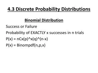
Cont. The mass function of binomial distribution: From the binomial formula, we can have = A random variable X is a binomial distribution if 1. The experiment consists of a fixed number n of identical trials. 2. Each trial only have two possible outcomes, that is the Bernoulli trials. 3. The probability p is constant from trial to trial. 4. The trials are independent. 5. X is the number of successes in n trails.
Example 4.9 Suppose that 10% of a large lot of apples are damaged. If four apples are randomly sampled from the lot, find the probability that exactly one apple is damaged. Find the probability that at least one apple in the sample of four is damaged. p(X=1) = P(X≥1)=1-P(X=0)=1-(1-0.1)4
Example 4.10 In a study of life lengths for a certain battery for laptop computers, researchers found that the probability that a battery life Y will exceed 5 hours is 0.12. If three such batteries are in use independent laptops, find the probability that only one of the batteries will last 5 hours or more. Let X be the number of batteries lasting 5 hours or more, then X follows the binomial distribution with p=0.12. So
E(X)=np Bernoulli random variables Y1, Y2, …, Yn, then V(X)=np(1-p) Bernoulli random variables Y1, Y2, …, Yn, then V
Example 4.11 Referring to Example 4.9, suppose that a customer is the one who randomly selects and then purchase the four apples. If an apple is damaged, the customer will complain. To keep the customers satisfied, the store has a policy of replacing any damaged apple and giving the customer a coupon for future purchases. The cost of this program has, through time, been found to be C=0.5X2, where X is the number of damaged apples in the purchase of four. Find the expected cost of the program when a customer randomly selects four apples from the lot. E(C) = E(0.5X2) = 0.5E(X2). Based on V(X)=E(X2)-E2(X), we have E(X2)=V(X)+E2(X)=np(1-p)+(np)2 = 4*0.1*0.9+(4*0.1)2=0.52, then E(X)=0.5*0.52=0.26.
Example 4.12 An industrial firm supplies 10 manufacturing plants with a certain chemical. The probability that any one firm will call in an order on a given day is 0.2, and this probability is the same for all 10 plants. Find the probability that, on the given day, the number of plants calling in orders is as follows: At most 3 At lest 3 Exactly 3. Let X be the number of plants that call in orders on the day in question, p=0.2, n=10. 1. P(X≤3)= 2. P(X≥3)=1-P(X≤2)=1-=1-0.678=0.322 3. P(X=3)=P(X≤3)-P(X≤2)=0.875-0.678=0.201.
Example 4.13 Every hospital has backup generators for critical systems should the electricity go out. Independent but identical backup are installed so that the probability that at least one system will operate correctly when on is no less than 0.99. Let n denote the number of backup generators in a hospital. How large must n be to achieve the specific probability of at least one generator operating, if p=0.95? P=0.8? Let X denote the number of correctly operating generators. P(X≥1)=1-P(X=0)=1-(1-p)n≥0.99 When p=0.95, 1-(1-0.95)n≥0.99 n=2, will satisfy the specification. When p=0.80, 1-(1-0.80)n≥0.99 n=3, will satisfy the specification.
Example 4.14 Virtually any process can be improved by the use of statistics, including the law. A much-publicized case that involved a debate about probability was the Collins case, which began in 1964. An incident of purse snatching in the Los Angeles area led to the arrest of Michael and Janet Collins. At their trial, an “expert” presented the following probabilities on characteristics possessed by the couple seen running from the crime. The chance that a couple had all of the specified characteristics together is 1 in 12 million. Because the Collinses had all of the specified characteristics, they must be guilty. What, if anything, is wrong with this line of reasoning? Man with beard 1/10 Blond woman ¼ Yellow car 1/10 Woman with ponytail 1/10 Manwith mustache 1/3 Interracial couple 1/1000
No background data are offered to support the probabilities used. The six events may not be independent each other, thus the probabilities can’t be multiplied. The wrong question is addressed. The proper question is “What is the probability that another such couple exists, given that we found one”. n=Number of couples who could have committed the crime p=probability that any couple possesses the six listed characteristics x=number of couples who possess the six characteristics.We know P(X=0)=(1-p)n, P(X=1)=np(1-p)n-1, P(X≥1)=1-(1-p)n. So the conditional probability is P(X>1|X≥1)=P(X>1)/P(X≥1) = Substituting p=1/(12Million) and n=12Million, we have P(X>1|X ≥1)=0.42, is much larger than the probability of seeing such a couple in the first place.