Download
1 / 31
310 likes | 414 Views
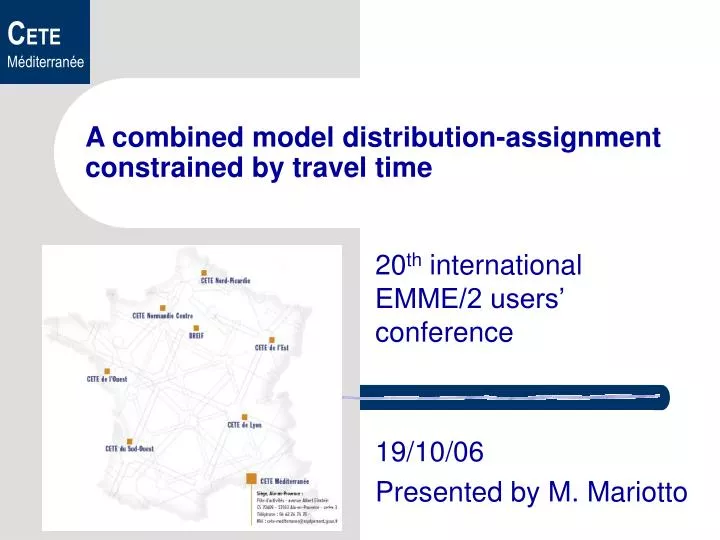
A combined model distribution-assignment constrained by travel time. 20 th international EMME/2 users’ conference 19/10/06 Presented by M. Mariotto. Who we are - n°1. The C.E.T.E. Méditerranée 1 / 7 technical centers of the French transport ministry

E N D
A combined model distribution-assignment constrained by travel time 20th international EMME/2 users’ conference 19/10/06 Presented by M. Mariotto
Who we are - n°1 • The C.E.T.E. Méditerranée • 1 / 7 technical centers of the French transport ministry • in charge of the East-Southern French regions (600 employees) • a consultant company working in the competitive sector • in the fields of : • Transports development, politics and planning • Environment, territories development, urban economy • Risks management • Road management • Civil engineering • Earth observation • Geotechnical works
Who we are - n°2 • My team • in charge of urban traffic studies and transport planning • in the field of modelling, 4 people (1 engineer and 3 technicians) working on : • model buildings • (monomodal models principally) • traffic studies and transport plans • (new facility effects for example, static and dynamic approach, but mainly with auto mode) • audit of model developments • (on multimodal models for instance) • development of new approaches • (2 studies with AIMSUN combined with former models developed on EMME/2)
Starting point - n°1 • Background • We are in charge of one of the models used to forecast urban traffic in Marseilles (around 1 million inhabitants) • Monomodal model with an equilibrium auto assignment of an aggregated matrix • In the frame of a work for the private company operating the only toll infrastructure in Marseilles, it was necessary to calibrate it in time (in order to update the optimal toll) • Possibility to assign depending on 2 users’ classes
Populations Jobs GENERATION Daily emissions assessed in motorized trips Daily attractions assessed in motorized trips DISTRIBUTION (1) OD matrices of daily motorized trips by 3 main purposes TIME OF DAY MODAL SPLIT 1 OD matrix aggregated in vehicles OD matrices of motorized trips for the evening peak hour given by purpose and mode VEHICLE OCCUPANCY ASSIGNMENT Reproduction of traffic for the evening peak hour (flows, travel time, path analyses …) (1) Entropic distribution model based on distance table calibrated for the 3 different trip purposes Starting point - n°2 • Model process overview
Starting point - n°3 • Calibration of the predicted vs observed flows (around 100 measurement points) • Calibration of the aggregated matrix in 10*10 zones • Calibration of travel times (it was in 1993 !) • Forecasts based on : • an increase of the total demand of 4% • an increase of the internal demand of 2% • tests done on future scenarios with or without new infrastructures
Starting point - n°4 • Model forecasts overview • Traffic simulations indicating benefits of a new express road, even for the internal demand : • Future scenario without the express road (in comparison with the actual scenario) • Increase of +66% on average travel time • Increase of +25% on average travel length • Increase of +77% on veh*h • Increase of +28% on veh*km • => + 4.5 km/h lost on average speed • Future scenario with the express road (in comparison with the actual scenario) • Smaller increase on average travel time (+49% / +66%) • A slightly higher increase on average travel length (+28% / +25%) • Smaller increase on veh*h (+56% / +77%) • A slightly higher increase on veh*km (+31% / +28%) • => + 2km/h gained on average speed in comparison with the situation without the new infrastructure
Starting point - n°5 • Targets • Drive access to activities • Socio-economic assessments based on the results of such studies • Models always indicate benefits associated with new facility • Traffic induction • Urban spreading questioning • Driving force • Economic approach in the field of individual time management • Zahavi researches and co • Stability observed locally (Marseilles) for motorized average travel time for evening peak hour
Starting point - n°6 • Issue • Analysis of the last household surveys • conclusions opposed to traffic forecasts : • For the past decade, observed data to conclude to : • non significant evolutions for average travel time • a rather stable average travel length • a higher rate for motorized mobilities evolution (conjectural) • an increase for veh*km due to mobility, but not due to a raise of average travel length
GENERATION Demand matrix Traffic assignment results DISTRIBUTION MODAL SPLIT ASSIGNMENT Starting point - n°7 • Approach principles • introduce an average travel time constraint • control distribution thanks to this constraint • feedback of assignment on distribution • aim : to calibrate the distribution model with an entropic formula depending on travel times resulting from assignment
matrix aggregated in vehicles for evening peak hour Vehicles emissions and attractions for the evening peak hour COMBINED ASSIGNMENT DISTRIBUTION MODEL CALIBRATION (2) Reproduction of traffic for the evening peak hour under the constraint on travel times (2) Entropic distribution model based on travel times Process implementation - n°1 • Modeling framework
Process implementation - n°2 • Algorithm based on : • Furness and Fratar method for distribution problem resolution under entropic model, • Frank and Wolf linear approximation method for solving equilibrium assignment problem under Wardrop principle, • Partial linear approximation of Frank and Wolf method for solving the combined trip assignment-distribution problem (S.P. Evans)
Process implementation - n°3 1/ Entropic distribution model depending on exp(-*free_flow_time) of emissions and attractions calculated formerly provides the first OD matrix (Gpq) 2/ Equilibrium assignment of this matrix gives the flows on segments. A travel time matrix is also calculated. 3/ Distribution based on the entropic model applied to the travel time matrix obtained at the previous step (assignment) gives a new OD matrix. 4/ The difference between step1 and step3 demand matrices entails to test the convergence of the iterative process. 5/ If the test fails, that is to say that the convergence is not enough, so the process has to continue by the successive averages method applied to the demand matrices (and flows as well) 6/ The assignment of the resulting matrix on a network pre-assigned with the resulting flows provides the travel time matrix Back to step 3 … Op Dp DISTRIBUTION MODEL (with fixed ) Gpq TEST Network codification Assignment algorithm Va Upq Global principle This process is known as convergent
Process implementation - n°4 • In practice, an algorithm implementing : • 2 iterative processes • The first one : • at fixed, research of convergence of the combined distribution-assignment processes • stopping criteria depending on the stability of the demand matrix resulting of the process between 2 steps • successive averages principle • introduction of a 3 D distribution with a travel times histogram
Process implementation - n°5 • The second one : • makes evolved with the postulate that the average travel time calculated at a given is a decreasing function of • stopping criteria depending on the proximity between the predicted average travel time and the observed value
Process implementation - n°6 Calcul of 0 (for instance 1/observed average travel time) And the observed travel times histogram for step0 Equilibrium assignment of the basic model we have in charge Travel time matrix New internal demand matrix Assignment0 volau Distribution 3D y Index function given travel times histogram Equilibrium assignment volau=new_volau x=x+1 volau no test1 New internal demand matrix New_volau Successive averages method on flows and demand x=0 yes Calcul of y+1 Calcul Travel time matrix (assignment 0) no test2 New internal demand matrix New volau New travel time matrix Distribution 3D with y yes Test1 = stability between two x step of the resulting demand Test2 = proximity with the observed average travel time
Process implementation - n°7 • A data panel not accurate enough • An average travel time calculated around 21.42 • A confidence level >20%
Process implementation - n°8 • The constraint controlling the test of the iterative calibration of is, not only the average travel time (which is not accurate enough), but also, the travel times histogram
Results - n°1 • Analysis of the process implementation • Research of and evolution of the average travel time
Results - n°2 • Analysis of the process implementation • Fast convergence of the combined processes
Results - n°3 • Analysis of the process implementation • A good reproduction of the travel times histogram whatever combined processes step
Differences between predicted flows of the combined processes at step1 with the predicted flows of the combined processes at step 15 Results - n°4 • Process implementation analysis • Evolution of predicted flows depending on the combined processes step • flow differences <2% (but it can reach a value around 200 veh/hps on some segments) • Other Traffic results differences <6% (veh*km ; veh*h)
Differences between combined processes predicted flows and step0 matrix assignment results Results - n°5 • Comparison between the combined processes results and the step0 matrix assignment results • Travel times histogram analysis (already discussed) • Traffic analysis assignment results :
Results - n°6 • Comparison between the combined processes results and the step0 matrix assignment results • Analysis of predicted vs observed flows
Differences between combined processes internal demand matrix and the step0 matrix Results - n°7 • Comparison between the combined processes results and the step0 matrix assignment results • Analysis of internal demand matrices
Results - n°8 • Comparison between the combined processes results and the step0 matrix assignment results • Analysis of other traffics assignments results • Average travel time : -15% • Average travel length : -2% • veh*h : -10% • veh*km : -3%
Results - n°9 • Comparative analysis on traffic forecasts between the combined processes results and the step0 matrix assignment results • Analysis on predicted flows
Results - n°10 • Comparative analysis on traffic forecasts between the combined processes results and the step0 matrix assignment results • Future scenario without the express road (in comparison with the actual scenario) • Average travel time constrained to be stable • A rather stable average travel length evolution (slight decrease) • Veh*km and veh*h decreasing slightly • Average speed stable between the future and the actual scenario • Future scenario with the express road (in comparison with the actual scenario) • Average travel time constrained to be stable • A rather stable average travel length evolution • A slight increase of the veh*km and veh*h • Average speed increased only by 1 km/h • => Minor benefits with the new facility
Back to the questions at stake • For now, work limited to a new distribution (emissions and attractions constrained by the totals of the step0 matrix) • A potential process to test urban spread, but with other researches • Feedback of assignment on distribution (for the internal matrix) • One way to take into account the effect of the limitation of the offer on the demand • A more centered matrix, future scenarios with less degradation of the traffic conditions • Combined processes non-necessarily indicate benefits for a new facility • Combined processes providing a mean to take into account the effects of a new infrastructure on reports with induction
Cautions and discussions - n°1 • Warnings : • Process experimented on the internal demand limited to a very urban perimeter • Monomodal aggregate model • Non accurate data • To go further : • Test sensitivity (offer, transport policies, demo-economic evolutions) • Comparisons with empirical formulae of traffic induction • What if the perimeter is larger ? • Working with emission and attraction totals calculated with a work on mobilities and modal split • Calibrate different for each trip purpose • What if the model is multimodal ?
Cautions and discussions - n°2 • A potential : • A mean to test new facilities in regard to drive access to activities and urban spread • Conclusions : • One help for decisions in a financial constrained world and with urban spreading for which parameters can no longer be exogenous (impact of offer on demand) • Bases for a work on accessibility • An approach entailing to a work on mobilities