FW364 Ecological Problem Solving
FW364 Ecological Problem Solving . Class 24: Competition. November 27, 2013. Recap from Last Class. dP 1 / dt = a 1 c 1 RP 1 – d 1 P 1. dP 2 / dt = a 2 c 2 RP 2 – d 2 P 2. Predator 1:. Predator 2:. From the chemostat experiment:. More TODAY. Rotifers have a R* = 40 μ g/L.


FW364 Ecological Problem Solving
E N D
Presentation Transcript
FW364 Ecological Problem Solving Class 24: Competition November 27, 2013
Recap from Last Class • dP1/dt= a1c1RP1 – d1P1 • dP2/dt= a2c2RP2 – d2P2 • Predator 1: • Predator 2: • From the chemostat experiment: • More TODAY • Rotifers have a R* = 40 μg/L • Daphnia have a R* = 20 μg/L • Daphnia wins! • Consumer with the lowest R* always wins • Rotifers will take early lead, but Daphnia will win at lower resource levels
Chemostat R* Experiment – Both Consumers . . . . . . . . . . . . . . . . . . . . . . . . . . . . . . • Rotifers do best at high resources . . . . . . . . . . . . . . . . . . • But when R drops below rotifer R* • (due to Daphnia consumption) • rotifers decline . . . . . . . . . . . . . . . . . . . . . . . . . . . . . • Daphnia win due to lower R* . . . . . . . Day 1 . Day 12 Day 21 . . . Rotifer Daphnia Biomass (μg/L) RR* Algae RD* Days
Competitive Exclusion Summary • To sum up • Giventhese assumptions: • a stable environment • competitors that are not equivalent (different R*) • a single resource • unlimited time • Then: • The species with the lowest minimum resource requirement (R*) • will eventually exclude all other competitors • Let’s look at some of the other assumptions we have made more closely
Competition Equation Assumptions • dP1/dt= a1c1RP1 – d1P1 • dP2/dt= a2c2RP2 – d2P2 • Predator 1: • Predator 2: • dR/dt= brR- drR – a1RP1 – a2RP2 • Resource: • Additional assumptions(from predator-prey models): • The consumer populations cannot exist if there are no resources • In the absence of both consumers, the resources grow exponentially • Consumers encounter prey randomly (“well-mixed” environment) • Consumers are insatiable (Type I functional response) • No age / stage structure • Consumers do not interact with each other except through consumption • (i.e., exploitative competition)
Competition Equation Assumptions • dP1/dt= a1c1RP1 – d1P1 • dP2/dt= a2c2RP2 – d2P2 • Predator 1: • Predator 2: • dR/dt= brR- drR – a1RP1 – a2RP2 • Resource: • Additional assumptions(from predator-prey models): • The consumer populations cannot exist if there are no resources • In the absence of both consumers, the resources grow exponentially • Consumers encounter prey randomly (“well-mixed” environment) • Consumers are insatiable (Type I functional response) • No age / stage structure • Consumers do not interact with each other except through consumption • (i.e., exploitative competition)
Adding Consumer Satiation Assumption 4: Consumers are insatiable • i.e., consumers eat the same proportion of the resource population (a) • no matter how many resources (R) there are • Type I functional response • To relax assumption, we can make the consumer feeding rate (aR) • a saturating function of the resource abundance • Type II functional response • Type II functional response Satiation • Type I functional response (linear) • high • aR • low • Let’s define an equation for Type II response • 0 • many • R
Adding Consumer Satiation • First, we need a new symbol for feeding rate: • Feeding rate: f • For a Type I functional response (linear): • f = aR • For a Type II functional response (saturating): • Where: fmax is the maximum feeding rate • h is the half-saturation constant • R is resource abundance • fmaxR • f= • R + h • Let’s look at a figure…
Adding Consumer Satiation • Where: fmax is the maximum feeding rate • h is the half-saturation constant • R is resource abundance • fmax = 5 • Consumer feeding rate approaches fmax at high resource abundance • fmaxR • f= • R + h
Adding Consumer Satiation • Where: fmax is the maximum feeding rate • h is the half-saturation constant • R is resource abundance • fmax = 5 • Challenge Question: • What is h for this figure? • fmaxR • f= • R + h • h is the value of R when the feeding rate is half of the maximum value • i.e., h is value of R whenf/fmax= 0.5
Adding Consumer Satiation • Where: fmax is the maximum feeding rate • h is the half-saturation constant • R is resource abundance • fmax = 5 • fmax = 5 and half of 5 is 2.5 • So, h is value of R when f is 2.5 • h = 2 • fmaxR • f= • R + h • 2 • h is the value of R when the feeding rate is half of the maximum value • i.e., h is value of R whenf/fmax= 0.5
Adding Consumer Satiation • Where: fmax is the maximum feeding rate • h is the half-saturation constant • R is resource abundance • fmax = 5 • A Type II functional response can apply to any type of consumer: • Carnivores, herbivores, parasites, and plants • Though plants do not eat (attack) resources, their growth still increases with resource abundance to some threshold rate • (i.e., until saturated with resources) • Let’s put the Type II response into our consumer growth equation (dP/dt) • fmaxR • f= • R + h • h is the value of R when the feeding rate is half of the maximum value • i.e., h is value of R whenf/fmax= 0.5
Type II Functional Response - Equation • dP/dt= acRP – dpP • Type I functional response: • dP/dt= caRP – dpP • Re-arrange to get aRadjacent: • dP/dt= cfP – dpP • Replace aR with f: • General equation that we can put any functional response (f) into: • dP/dt= cfP – dpP • With Type II functional response: • fmaxR • f= • R + h • cfmaxRP • dP/dt= • – dpP • Plug f into general equation: • R + h • Equation for consumer growth with a Type II functional response
R* for Type II Functional Response • Our functional response has changed, • so we need to a new R* equation • i.e., R* for Type II response • R* occurs at steady-state, • so set dP/dt= 0 • Solve for R* • cfmaxR*P* • = dpP* • R* + h • dph • cfmaxRP • cfmaxR*P* • dP/dt= • – dpP • 0= • – dpP* • R* = • R + h • R* + h • c fmax - dp • …a whole lot of algebra you do in Lab 10…
R* for Type II Functional Response • Conclusions: • With a Type II functional response: • R* depends on consumer death rate, half saturation constant, • conversion efficiency, and max feeding rate • If consumer death rate increases, R* increases • If consumer half saturation constant increases, R* increases • If conversion efficiency increases, R* decreases • If max feeding rate increases, R* decreases • dph • R* = • c fmax - dp
Saturation & Consumer Birth Rate • That was a lot about feeding rate… • … need to get back to competition • To do that, need to make a crucial link • between consumer feeding rate and birth rate • R* is key for competition… and R* depends on dp • Competition winner is the consumer alive • at steady state … i.e., when bp = dp • Knowing birth rate of consumer is important for determining competition outcome • dph • R* = • c fmax - dp • Let’s look at how a saturating feeding rate affects consumer birth rate
Saturation & Consumer Birth Rate • Type II functional response: • Minor re-arrangement: • This is all equivalent to our consumer birth rate • i.e., consumers are born by feeding on prey • cfmaxRP • cfmaxR • Consumer birth rate function should curve the same as the feeding rate, • since birth rate is just feeding rate multiplied by a constant • (conversion efficiency) • dP/dt= • dP/dt= • – dpP • P – dpP • R + h • R + h
Saturation & Consumer Birth Rate • fmax • high • Feeding rate (f) • high • Resource abundance (R) • bmax • high • birth rate (bp) • high • Resource abundance (R)
Saturation & Consumer Birth Rate • fmax • high • Consumer birth rate increases with resource abundance • to a threshold rate, bmax • (threshold birth rate is due to feeding rate hitting threshold) • h, the half-saturation constant, still applies: • h is the value of R when the birth rate is half of the maximum value • Feeding rate (f) • high • Resource abundance (R) • bmax • high • birth rate (bp) • high • Resource abundance (R)
Saturation & Consumer Death Rate • So that’s how consumer birth rate changes with resource density… • …now on to death rate • We have been making an (implicit) assumption about • how consumer death rate changes with resource density • We’ve been assuming that the consumer death rate is a constant (dp) • i.e., that the consumer death rate does NOT change with resource density • To plot this assumption on a figure… • cfmaxRP • dP/dt= • – dpP • R + h
Saturation & Consumer Death Rate • Consumer death rate is just a straight line at any value along the y-axis • high • Death rate • death rate (dp) • high • Resource abundance (R) • If we combine the death rate function with the birth rate curve…
Saturation & Consumer Death Rate • Consumer death rate is just a straight line at any value along the y-axis • Birth rate • high • Death rate • birth rate (bp) • death rate (dp) • high • Resource abundance (R) • If we combine the death rate function with the birth rate curve… • we have a useful trick for graphically determining R* for a consumer… • (consumer birth rate and death rate must be plotted on the same scale!)
Graphical approach to R* • Birth rate • high • Death rate • birth rate (bp) • death rate (dp) • high • Resource abundance (R) • Challenge question: • A special point on this figure represents steady state… • Where is this point?
Graphical approach to R* • Birth rate • high • Death rate • birth rate (bp) • death rate (dp) • Steady state when b = d • high • Resource abundance (R) • Challenge question: • A special point on this figure represents steady state… • Where is this point?
Graphical approach to R* • Birth rate • high • Death rate • birth rate (bp) • death rate (dp) • Steady state when b = d • R* • high • Resource abundance (R) • KEY feature of this graph: • The resource abundance (i.e., value on x-axis) at the steady state point (i.e., intersection of b and d functions) is R*!
Graphical approach to R* • Birth rate • high • Death rate • birth rate (bp) • death rate (dp) • Steady state when b = d • R* • high • Resource abundance (R) • Key application: • If we plot the birth and death rates of two competing species on same figure, we can determine which consumer will win based on who has the lower R*
Graphical Approach to R* • First, one more question for single consumer: • high • Death rate • Birth rate • birth rate (bp) • death rate (dp) • high • Resource abundance (R) • Quick Challenge Question: • What happens if the death rate is higher than the birth rate?
Graphical Approach to R* • First, one more question for single consumer: • high • Death rate • Birth rate • birth rate (bp) • death rate (dp) • high • Resource abundance (R) • What happens if the death rate is higher than the birth rate? • Consumer goes extinct, even without the competitor • Now let’s look at resource competition
Graphical R* & Competition • Outline: • Look at four graphical cases of two-species competition • (competition with Type II functional response) • Consumers will have: • Case 1: Different birth rates, same death rate and h • Case 2: Different birth rates and death rates, same h • Case 3: Different birth rates, same death rates, different h • Case 4: Different birth rates, same death rate, different h w/ twist • For each case, we’ll determine competition winner
Case 1: Effect of different birth rates • b1 • b2 • d1d2 • Consumer 1 has a higher birth rate than Consumer 2 at all R levels (b1 > b2) • Both consumers have same death rate, d1 = d2 • Monod curves never cross • Who wins?
Case 1: Effect of different birth rates • b1 • b2 • d1d2 • R1* • R2* • Consumer 1 has a higher birth rate than Consumer 2 at all R levels (b1 > b2) • Both consumers have same death rate, d1 = d2 • Monod curves never cross • Higher birth rate makes better competitor • Consumer 1 wins: R1* < R2*
Case 2A: Effect of different death rates • b1 • d1 • b2 • d2 • Consumer 1 has a higher birth rate than Consumer 2 at all R levels (b1 > b2) • Consumer 1 has a higher death rate than Consumer 2 (d1> d2) • Monod curves never cross • Who wins?
Case 2A: Effect of different death rates • b1 • d1 • b2 • d2 • R2* • R1* • Consumer 1 has a higher birth rate than Consumer 2 at all R levels (b1 > b2) • Consumer 1 has a higher death rate than Consumer 2 (d1> d2) • Monod curves never cross • Lower death rate makes better competitor • Consumer 2 wins: R2* < R1*
Case 2B: Effect of different death rates • b1 • b2 • d2 • d1 • Consumer 1 has a higher birth rate than Consumer 2 at all R levels (b1 > b2) • Consumer 2 has a higher death rate than Consumer 1 (d2> d1) • Monod curves never cross • Who wins?
Case 2B: Effect of different death rates • b1 • b2 • d2 • d1 • R2* • R1* • Consumer 1 has a higher birth rate than Consumer 2 at all R levels (b1 > b2) • Consumer 2 has a higher death rate than Consumer 1 (d2> d1) • Monod curves never cross • Consumer 1 wins: R1* < R2* • Lower death rate makes better competitor
Case 3: Effect of different h • b1b2 • b1 • At very high resource density • b2 • d1d2 • Both consumers have same maximum birth rate, b1max = b2max • Both consumers have same death rate, d1 = d2 • Consumer 1 has a lower h ( Consumer 1 approaches bmax at lower R) • Who wins?
Case 3: Effect of different h • b1b2 • b1 • At very high resource density • b2 • d1d2 • R1* • R2* • Both consumers have same maximum birth rate, b1 = b2 • Both consumers have same death rate, d1 = d2 • Consumer 1 has a lower h ( Consumer 1 approaches bmax at lower R) • Consumer 1 wins: R1* < R2* • Lower h makes better competitor
Graphical R* & Competition Summary • What makes a better competitor(i.e., lower R*)? • Higher birth rate • Lower death rate • Lower h • We reached the same conclusions looking at R* equation • If consumer death rate increases, R* increases • so lower dp makes better competitor • If consumer half saturation constant increases, R* increases • so lower h makes better competitor • If conversion efficiency increases, R* decreases • If max feeding rate increases, R* decreases • Birth rate is just conversion efficiency * feeding rate, • so higher birth rate makes better competitor • dph • R* = • c fmax - dp
Graphical R* & Competition Summary • What makes a better competitor(i.e., lower R*)? • Higher birth rate • Lower death rate • Lower h • Does this perfect competitor exist in nature? • Not really… there are always trade-offs in nature • e.g., high max birth rate requires more resources, • foraging exposes consumers to predation, • and so high bmax associated with high death rates • High birth rate rabbit takes risks to forage