Download
1 / 222
2.23k likes | 2.33k Views
The Population Haplotyping problem. NOTATION : each SNP only two values in a population ( bio ). Call them 0 and 1 . Also , call * the fact that a site is heterozygous. HAPLOTYPE : string over 0, 1 GENOTYPE : string over 0, 1, *

E N D
NOTATION: each SNP onlytwovalues in a population (bio). Call them0and 1. Also, call *the factthat a site isheterozygous HAPLOTYPE: string over 0, 1 GENOTYPE: string over 0, 1, * where0={0}, 1={1}, *={0,1} 01 0* 00 10 1* 11 11 11 11 01 ** 10 10 *0 00 10 10 10 *0 10 00
ALGEBRA OF HAPLOTYPES: 0 + 0 = --- 0 1 + 1 = --- 1 0 + 1 + 1 = 0 = --- --- * * Heterozygous (ambiguous) sites Homozygous sites 01 00 0* 10 1* 11 01 ** 11 10 ** 00 10 00 10 *0 10 10
Phasing the alleles 11101 10000 11100 10001 11001 10100 11000 10101 1**0* For k heterozygous (ambiguous) sites, there are 2k-1 possible phasings
THE PHASING (or HAPLOTYPING) PROBLEM It is too expensive to determine haplotypes directly Much cheaper to determine genotypes, and then infer haplotypes in silico: Given genotypes of k individuals, determine the phasings of all heterozygous sites. This yields a set H, of (at most) 2k haplotypes. H is a resolution of G.
The input is GENOTYPE data *1**1 11**1 11011 ****1 00011 INPUT: G = { 11**1, ****1, 11011, *1**1, 00011 }
The input is GENOTYPE data 11011 01101 *1**1 11011 11101 11**1 11011 11011 11011 00011 11101 ****1 00011 00011 00011 INPUT: G = { 11**1, ****1, 11011, *1**1, 00011 } OUTPUT: H = { 11011, 11101, 00011, 01101} Each genotype is resolved by two haplotypes We will define some objectives for H
OBJECTIVES -without objectives/constraints, the haplotyping problem would be (mathematically)trivial E.g., always put 0 above and 1 below **0*1 00001 11011 1*0** 10000 11011 -the objectives/constraints must be “driven by biology”
OBJECTIVES 1°) Clark’s inference rule 2°) Perfect Phylogeny 3°) DiseaseAssociation 4°) (parsimony): minimize |H|
1st Obj: Clark’s rule
Inference Rule for a compatible pair h , g known haplotypeh 1011001011 + ?????????? = 1**1001*1* known (ambiguos) genotype g
Inference Rule for a compatible pair h , g known haplotypeh 1011001011 + 1101001110 = 1**1001*1* new (derived) haplotype h’ known (ambiguos) genotype g We write h + h’ = g
1st Objective (Clark, 1990) 1. Start with H = “bootstrap” haplotypes 2. while Clark’s rule applies to a pair (h, g) in H x G 3. apply the rule to any such (h, g) obtaining h’ 4. set H = H + {h’} and G = G - {g} 5. end while
1st Objective (Clark, 1990) 1. Start with H = “bootstrap” haplotypes 2. while Clark’s rule applies to a pair (h, g) in H x G 3. apply the rule to any such (h, g) obtaining h’ 4. set H = H + {h’} and G = G - {g} 5. end while If, at end, G is empty, SUCCESS, otherwise FAILURE Step 3 is non-deterministic
1st Objective (Clark, 1990) 1. Start with H = “bootstrap” haplotypes 2. while Clark’s rule applies to a pair (h, g) in H x G 3. apply the rule to any such (h, g) obtaining h’ 4. set H = H + {h’} and G = G - {g} 5. end while If, at end, G is empty, SUCCESS, otherwise FAILURE Step 3 is non-deterministic 0000 1000 **00 11**
1st Objective (Clark, 1990) 1. Start with H = “bootstrap” haplotypes 2. while Clark’s rule applies to a pair (h, g) in H x G 3. apply the rule to any such (h, g) obtaining h’ 4. set H = H + {h’} and G = G - {g} 5. end while If, at end, G is empty, SUCCESS, otherwise FAILURE Step 3 is non-deterministic 0000 1000 **00 11** 1100
1st Objective (Clark, 1990) 1. Start with H = “bootstrap” haplotypes 2. while Clark’s rule applies to a pair (h, g) in H x G 3. apply the rule to any such (h, g) obtaining h’ 4. set H = H + {h’} and G = G - {g} 5. end while If, at end, G is empty, SUCCESS, otherwise FAILURE Step 3 is non-deterministic 0000 1000 **00 11** 1100 SUCCESS 1111
1st Objective (Clark, 1990) 1. Start with H = “bootstrap” haplotypes 2. while Clark’s rule applies to a pair (h, g) in H x G 3. apply the rule to any such (h, g) obtaining h’ 4. set H = H + {h’} and G = G - {g} 5. end while If, at end, G is empty, SUCCESS, otherwise FAILURE Step 3 is non-deterministic 0000 1000 **00 11**
1st Objective (Clark, 1990) 1. Start with H = “bootstrap” haplotypes 2. while Clark’s rule applies to a pair (h, g) in H x G 3. apply the rule to any such (h, g) obtaining h’ 4. set H = H + {h’} and G = G - {g} 5. end while If, at end, G is empty, SUCCESS, otherwise FAILURE Step 3 is non-deterministic 0000 1000 **00 11** 0100
1st Objective (Clark, 1990) 1. Start with H = “bootstrap” haplotypes 2. while Clark’s rule applies to a pair (h, g) in H x G 3. apply the rule to any such (h, g) obtaining h’ 4. set H = H + {h’} and G = G - {g} 5. end while If, at end, G is empty, SUCCESS, otherwise FAILURE Step 3 is non-deterministic 0000 1000 **00 11** 0100 FAILURE (can’t resolve 1122 )
1st Objective (Clark, 1990) 1. Start with H = “bootstrap” haplotypes 2. while Clark’s rule applies to a pair (h, g) in H x G 3. apply the rule to any such (h, g) obtaining h’ 4. set H = H + {h’} and G = G - {g} 5. end while If, at end, G is empty, SUCCESS, otherwise FAILURE Step 3 is non-deterministic: the algorithm could end without explaining all genotypes even if an explanation was possible. The number of genotypes solved depends on order of application. OBJ: find order of application rule that leaves the fewest elements in G
The problem was studied by Gusfield (ISMB 2000, and Journal of Comp. Biol., 2001) - problem is APX-hard - it corresponds to finding largest forest in a graph with haplotypes as nodes and arcs for possible derivations -solved via ILP of exponential-size (practical for small real instances)
2nd Obj: Perfect Phylogeny
- Parsimony does not take into account mutations/evolution of haplotypes - parsimony is very relialable on “small” haplotype blocks - when haplotypes are large (span several SNPs, we should consider evolutionionary events and recombination) - the cleanest model for evolution is the perfect phylogeny
3rd objective is based on perfect phylogeny - A phylogeny expalains set of binary features (e.g. flies, has fur…) with a tree - Leaf nodes are labeled with species - Each feature labels an edge leading to a subtree that possesses it
3rd objective is based on perfect phylogeny - A phylogeny expalains set of binary features (e.g. flies, has fur…) with a tree - Leaf nodes are labeled with species - Each feature labels an edge leading to a subtree that possesses it has 2 legs has tail flies
But…a new species may come along so that no Perfect phylogeny is possible… - A phylogeny expalains set of binary features (e.g. flies, has fur…) with a tree - Leaf nodes are labeled with species - Each feature labels an edge leading to a subtree that possesses it has 2 legs has tail flies
flies two legs tail Human 1 0 0 Mouse 0 1 0 Spider 0 0 0 Eagle 1 0 1 Theorem: such matrix has p.p. iff there is not a 00 4x2 minor 10 01 11
flies two legs tail Human 1 0 0 Mouse 0 1 0 Spider 0 0 0 Eagle 1 0 1 Mickey mouse 1 1 0 Theorem: such matrix has p.p. iff there is not a 00 4x2 minor 10 01 11
We can consider each SNP as a binary feature Objective: We want the solution to admit a perfect phylogeny (Rationale : we assume haplotypes have evolved independently along a tree)
We can consider each SNP as a binary feature Objective: We want the solution to admit a perfect phylogeny (Rationale : we assume haplotypes have evolved independently along a tree) 0 1 * 0 * 1 0 * * 0 * 0
We can consider each SNP as a binary feature Objective: We want the solution to admit a perfect phylogeny (Rationale : we assume haplotypes have evolved independently along a tree) 0 1 0 0 0 1 1 0 1 1 0 1 0 1 0 0 1 0 0 0 0 0 1 0 0 1 * 0 * 1 0 * * 0 * 0
We can consider each SNP as a binary feature Objective: We want the solution to admit a perfect phylogeny (Rationale : we assume haplotypes have evolved independently along a tree) 0 1 0 0 0 1 1 0 1 1 0 1 0 1 0 0 1 0 0 0 0 0 1 0 0 1 * 0 * 1 0 * * 0 * 0 NOT a perfect phylogeny solution !
We can consider each SNP as a binary feature Objective: We want the solution to admit a perfect phylogeny (Rationale : we assume haplotypes have evolved independently along a tree) 0 1 * 0 0 1 0 * 0 0 0 *
We can consider each SNP as a binary feature Objective: We want the solution to admit a perfect phylogeny (Rationale : we assume haplotypes have evolved independently along a tree) 0 1 0 0 0 1 1 0 0 1 0 0 1 1 0 1 0 0 0 0 0 0 0 1 0 1 * 0 0 1 0 * 0 0 0 * A perfect phylogeny
Theorem: The Perfect Phylogeny Haplotyping problem is polynomial
Theorem: The Perfect Phylogeny Haplotyping problem is polynomial Algorithms are of combinatorial nature - There is a graph for which SNPs are columns and edges are of two types (forced and free) - forced edges connect pairs of SNPs that must be phased in the same way ** 00 + 11 or ** 01 + 10 - a complex visit of the graph decides how to phase free SNPs
3rd Obj: Disease Association
Some diseases may be due to a gene which has “faulty” configurations RECESSIVE DISEASE (e.g. cystic fibrosis, sickle cell anemia): to be diseased one must have both copies faulty. With one copy one is a carrier of the disease DOMINANT DISEASE (e.g. Huntington’s disease, Marfan’s syndrome): to be diseased it is enough to have one faulty copy Two individuals of which one is healthy and the other diseased may have the same genotype. The explanation of the disease lies in a difference in their haplotypes
11**1 *1**1 0*011 11**1 0**01 00011 INPUT: GD = {11**1,*1**1,0*011}, GH ={11**1,0**01,00011}
11011 01101 11011 11101 01011 00011 11**1 *1**1 0*011 11001 11111 01101 00001 00011 00011 11**1 0**01 00011 INPUT: GD = {11**1,*1**1,0*011}, GH ={11**1,0**01,00011} OUTPUT: H = { 11011,01011,00001,11111,11101,00011,01101} H contains HD, s.t. each diseased has >=1 haplotype in HD and each healty none
Theorem 1 is proved via a reduction from 3 SAT Theorem 2 has a mathematical proof (coloring argument) with little relation to biology: There is R (depending on input) s.t. a haplotype is healthy if the sum of its bits is congruent to R modulo 3 This means the model must be refined!
4th Obj: MaxParsimony See separate slides…
Summary: - haplotyping in-silico needed for economical reasons - several objectives, all biologically driven - nice combinatorial problems (mostly due to binary nature of SNPs) - these problems are technology-dependant and may become obsolete (hopefully after we have retired)
111 111 011 101 011 000 111 111 010 001 010 011 022 222 012 221 222 011 012 022 022 211 111 012
2nd Objective (parsimony) : minimize |H|
1. The problem is APX-Hard Reduction from VERTEX-COVER
B A C D E