Download

1 / 23
230 likes | 399 Views
GIS based calculations for Lake/Water surface evaporation in the state of Texas. By: Paramjit Chibber Texas A & M University. Index. 1)Importance of evaporation in Reservoirs. 2)Data collection and completion. 3)Methodology involved. 4)Limitations. Importance of Evaporation.

E N D
GIS based calculations for Lake/Water surface evaporation in the state of Texas. By: Paramjit Chibber Texas A & M University.
Index 1)Importance of evaporation in Reservoirs. 2)Data collection and completion. 3)Methodology involved. 4)Limitations.
Importance of Evaporation. Def : Process by which water changes from the liquid or the solid state into gaseous state. (Ref:Merrill Bernard et. Al.). Storage :-. 1)Wide shallow reservoirs. 2)Deep narrow reservoirs. Note : Effects more prominent in tropical countries where annual. Evaporation sometimes exceeds Precipitation.
Measurement of water surface evaporation. Pan Evaporation Method : A circular pan of 4 Ft. diameter and 10 inches deep and is exposed on a wooden platform. Eo = cEp. Eo =Lake Evaporation. C = Pan evaporation coefficient. Ep = Pan evaporation.
Data Collection and Completion. Datasets Used: 1)Pan Evaporation at Gage Stations (NWS Hydrologic Research Lab). 2)Pan Evaporation in different Quadrangles (TWDB). 3)Reservoirs and Counties Datasets (TNRIS). 4)Pan Evaporation Coefficients (TWDB)
Raw Data NAME=DAINGERFIELD 9 S LAT= 32.92 LON= 94.72 ELEV= 300 <- 1960 -> <- 1970 -> <- 1980 -> <- 1990 -> 01234 56789 01234 56789 01234 56789 01234 56789 778C9 99C8C CC898 C9652 89-74 59878 86-85 75487 JAN C88C8 89CC8 CCCC9 7C983 87677 47764 978-6 87779 FEB
After this for all gage stations complete the datasets (Ep) for the year 1968.Following the same procedure complete the datasets for other years i.e 1958, 1978,1988,and 1998 as well. Now in excel spread sheet do the evaporation calculations at all gage stations using pan evaporation coefficients.
Up till last step we have calculated the water surface evaporation at all gage stations. NOW : Add Texas boundary theme. Add gage stations theme. OBSERVATION : One gage station found to be out side the boundary. SOLUTION : Buffer the boundary of Texas.
Methodology • Thiessen polygons: In this method polygons of same evaporation are generated 2) Grid method : In this method grids are created to measure evaporation.
Thiessen polygons: Create thiessen polygons with gage stations, considering buffered outer boundary.
Now Intersect “reservoirs” with the “thiessen polygons”. Update Areas of the intersected reservoirs. Add field Ev(AcFt). Fill up the Ev(AcFt) field. Ev(AcFt) = Area*Annual Evaporation (in inches) *247.1057/12000000. Note : After this step Annual evaporation of all the intersected polygons is known.
Now • Dissolve the intersected polygons (taking Reservoir# as the key attribute). • Look at the statistics for Ev(Acft) field. • Sum Ev(AcFt) gives annual evaporation.
Following the same steps find out evaporation for other years.Year :1958 1968 1978 1988 1998Evaporation (Acre Ft) : 11475752 11462713 14315370 12117721 12029697
2) Grid Method :This method converts point data into a grid or surface data.
Now “Summarize zones” to get the mean evaporation (in inches) Add Field Ev_gr(AcFt). Fill the Ev_gr(AcFt) with Ev_gr(AcFt) = Mean*Area*247.1057/12000000. “Statistics “of Ev_gr(AcFt) inform of the Annual evaporation.
Following the same steps find out evaporation for other years.Year 1958 1968 1978 1988 1998Evaporation (AcFt) : 12008612 10766627 12574776 12174579 12070145
Limitations. With Grid method it is observed that we can sometimes get wrong data.The possible reasons might be : Data not available at all gage stations. Original dataset incomplete.