Visual Object Recognition
This presentation delves into object recognition, highlighting the limitations of global representations and advocating for a focus on distinctive local features to enhance robustness against occlusions, articulations, and intra-category variations. Key topics include detection with global appearance, local invariant features, interest points detection, and the use of visual words for indexing and categorization. The talk covers challenges within the field and explores research directions, including the utilization of various existing detectors like Hessian and Harris, as well as local descriptors for improved accuracy.

Visual Object Recognition
E N D
Presentation Transcript
Visual Object Recognition Bastian Leibe & Computer Vision Laboratory ETH Zurich Chicago, 14.07.2008 Kristen Grauman Department of Computer Sciences University of Texas in Austin
Outline Detection with Global Appearance & Sliding Windows Local Invariant Features: Detection & Description Specific Object Recognition with Local Features ― Coffee Break ― Visual Words: Indexing, Bags of Words Categorization Matching Local Features Part-Based Models for Categorization Current Challenges and Research Directions 2 K. Grauman, B. Leibe
Motivation • Global representations have major limitations • Instead, describe and match only local regions • Increased robustness to • Occlusions • Articulation • Intra-category variations K. Grauman, B. Leibe
Approach 1. Find a set of distinctive key- points 2. Define a region around each keypoint A1 B3 3. Extract and normalize the region content A2 A3 B2 B1 Similarity measure 4. Compute a local descriptor from the normalized region N pixels e.g.color e.g.color 5. Match local descriptors N pixels K. Grauman, B. Leibe
Requirements • Region extraction needs to be repeatable and precise • Translation, rotation, scale changes • (Limited out-of-plane (affine) transformations) • Lighting variations • We need a sufficient number of regions to cover the object • The regions should contain “interesting” structure K. Grauman, B. Leibe
Many Existing Detectors Available • Hessian & Harris [Beaudet ‘78], [Harris ‘88] • Laplacian, DoG [Lindeberg ‘98], [Lowe 1999] • Harris-/Hessian-Laplace[Mikolajczyk & Schmid ‘01] • Harris-/Hessian-Affine [Mikolajczyk & Schmid ‘04] • EBR and IBR [Tuytelaars & Van Gool ‘04] • MSER[Matas ‘02] • Salient Regions [Kadir & Brady ‘01] • Others… K. Grauman, B. Leibe
Keypoint Localization • Goals: • Repeatable detection • Precise localization • Interesting content Look for two-dimensional signal changes K. Grauman, B. Leibe
Hessian Detector [Beaudet78] • Hessian determinant Ixx Iyy Ixy Intuition: Search for strongderivatives in two orthogonal directions K. Grauman, B. Leibe
Hessian Detector [Beaudet78] • Hessian determinant Ixx Iyy Ixy In Matlab: K. Grauman, B. Leibe
Hessian Detector – Responses [Beaudet78] Effect: Responses mainly on corners and strongly textured areas.
Harris Detector [Harris88] • Second moment matrix(autocorrelation matrix) Intuition: Search for local neighborhoods where the image content has two main directions (eigenvectors). K. Grauman, B. Leibe
Ix Iy Harris Detector [Harris88] • Second moment matrix(autocorrelation matrix) 1. Image derivatives Iy2 IxIy Ix2 2. Square of derivatives Iy 3. Gaussian filter g(sI) g(Ix2) g(Iy2) g(IxIy) 4. Cornerness function – both eigenvalues are strong g(IxIy) har 5. Non-maxima suppression
Harris Detector – Responses [Harris88] Effect: A very precise corner detector.
Automatic Scale Selection Same operator responses if the patch contains the same image up to scale factorHow to find corresponding patch sizes? K. Grauman, B. Leibe
Automatic Scale Selection • Function responses for increasing scale (scale signature) K. Grauman, B. Leibe
Automatic Scale Selection • Function responses for increasing scale (scale signature) K. Grauman, B. Leibe
Automatic Scale Selection • Function responses for increasing scale (scale signature) K. Grauman, B. Leibe
Automatic Scale Selection • Function responses for increasing scale (scale signature) K. Grauman, B. Leibe
Automatic Scale Selection • Function responses for increasing scale (scale signature) K. Grauman, B. Leibe
Automatic Scale Selection • Function responses for increasing scale (scale signature) K. Grauman, B. Leibe
What Is A Useful Signature Function? • Laplacian-of-Gaussian = “blob” detector K. Grauman, B. Leibe
Laplacian-of-Gaussian (LoG) • Local maxima in scale space of Laplacian-of-Gaussian s5 s4 s3 s2 List of(x, y, s) s K. Grauman, B. Leibe
Results: Laplacian-of-Gaussian K. Grauman, B. Leibe
Difference-of-Gaussian (DoG) • Difference of Gaussians as approximation of theLaplacian-of-Gaussian = - K. Grauman, B. Leibe
DoG – Efficient Computation • Computation in Gaussian scale pyramid Sampling withstep s4=2 s s s s Original image K. Grauman, B. Leibe
Results: Lowe’s DoG K. Grauman, B. Leibe
Harris-Laplace [Mikolajczyk ‘01] • Initialization: Multiscale Harris corner detection s4 s3 s2 s Computing Harris function Detecting local maxima
Harris-Laplace [Mikolajczyk ‘01] • Initialization: Multiscale Harris corner detection • Scale selection based on Laplacian(same procedure with Hessian Hessian-Laplace) Harris points Harris-Laplace points K. Grauman, B. Leibe
Maximally Stable Extremal Regions [Matas ‘02] • Based on Watershed segmentation algorithm • Select regions that stay stable over a large parameter range K. Grauman, B. Leibe
Example Results: MSER K. Grauman, B. Leibe
You Can Try It At Home… • For most local feature detectors, executables are available online: • http://robots.ox.ac.uk/~vgg/research/affine • http://www.cs.ubc.ca/~lowe/keypoints/ • http://www.vision.ee.ethz.ch/~surf K. Grauman, B. Leibe
p 2 0 Orientation Normalization • Compute orientation histogram • Select dominant orientation • Normalize: rotate to fixed orientation [Lowe, SIFT, 1999] T. Tuytelaars, B. Leibe
Local Descriptors • The ideal descriptor should be • Repeatable • Distinctive • Compact • Efficient • Most available descriptors focus on edge/gradient information • Capture texture information • Color still relatively seldomly used (more suitable for homogenous regions) K. Grauman, B. Leibe
Local Descriptors: SIFT Descriptor • Histogram of oriented gradients • Captures important texture information • Robust to small translations / affine deformations [Lowe, ICCV 1999] K. Grauman, B. Leibe
Local Descriptors: SURF • Fast approximation of SIFT idea • Efficient computation by 2D box filters & integral images 6 times faster than SIFT • Equivalent quality for object identification • GPU implementation available • Feature extraction @ 100Hz(detector + descriptor, 640×480 img) • http://www.vision.ee.ethz.ch/~surf [Bay, ECCV’06], [Cornelis, CVGPU’08] K. Grauman, B. Leibe
Local Descriptors: Shape Context Count the number of points inside each bin, e.g.: Count = 4 ... Count = 10 Log-polar binning: more precision for nearby points, more flexibility for farther points. Belongie & Malik, ICCV 2001 K. Grauman, B. Leibe
Local Descriptors: Geometric Blur Compute edges at four orientations Extract a patch in each channel ~ Apply spatially varying blur and sub-sample Example descriptor (Idealized signal) Berg & Malik, CVPR 2001 K. Grauman, B. Leibe
So, What Local Features Should I Use? • There have been extensive evaluations/comparisons • [Mikolajczyk et al., IJCV’05, PAMI’05] • All detectors/descriptors shown here work well • Best choice often application dependent • MSER works well for buildings and printed things • Harris-/Hessian-Laplace/DoG work well for many natural categories • More features are better • Combining several detectors often helps K. Grauman, B. Leibe
Outline Detection with Global Appearance & Sliding Windows Local Invariant Features: Detection & Description Specific Object Recognition with Local Features ― Coffee Break ― Visual Words: Indexing, Bags of Words Categorization Matching Local Features Part-Based Models for Categorization Current Challenges and Research Directions 44 K. Grauman, B. Leibe