Download
1 / 33
330 likes | 355 Views
Learn the fundamentals of SPM and fMRI modeling, from pre-processing steps like realignment and normalization to inferential techniques such as contrasts. Understand the general linear model and how it fits imaging data, enabling the identification of voxel activity patterns. Discover the process of designing and fitting statistical models to fMRI data, with a focus on contrasts and model inference. Gain insights into regressor construction, basis functions, and contrast guidelines for effective model specification.

E N D
SPM and (e)fMRI Christopher Benjamin
SPM • Today: basics from eFMRI perspective. • Pre-processing • Modeling: Specification & general linear model • Inference: Contrasts • Overview of process. • Please note to illustrate points I’ve included content from sources including Human Brain Function, others’ web powerpoints (see final slide for credits).
SPM • Pre-processing • Modeling: Specification & general linear model • Inference: Contrasts
Image pre-processing (1) Very briefly, after file extraction, NFTI… • Realignment: spatially align images. • Slice-timing correction: temporal alignment. • Coregistration: spatially registers the structural image to the functional images.
Image pre-processing (2) 4. Segmentation: tissue types. 5. Normalisation: Moves all images to a specific space – e.g. structural image, MNI-152. 6. Smoothing: smooth data, making it more normal (assumptions of later analysis). • Note: this processing sequence is from the SPM (e)fMRI manual example. • Manually or by batch script.
SPM • Pre-processing • Modeling: Specification & general linear model • Inference: Contrasts
Modeling: SPM and the general linear model • Each fMRI image yields a matrix of activation data. • Aim: identify voxels that behave as we’d expect. • We have: • A single time series of data for each voxel (Y values). • A set of expectations about what variables determine activity (X values).
Formally, the general linear model: Y = b1X1 + b2X2 …+ bNXN + e • b coefficients are calculated for each voxel (Ordinary Least Squares or Maximum Likelihood estimates). • Correlation of bX combination reflects strength of X’s influence on activity.
The model represented visually amplitude • General Linear Model • fitting • statistical image time Statistical image (SPM) Temporal series fMRI voxel time course Adapted from Poline (2005)
Regression example -10 0 10 90 100 110 90 100 110 -2 0 2 b2 b1 b2 = 100 b1 = 1 Fit the GLM Mean value voxel time series box-car reference f’n + + = Adapted from Poline (2005)
The model visually b2 = b1 + + error Y es = + + ´ ´ X 1 b1 b2 Adapted from Poline (2005)
b1 b2 ´ Y = X b + e The visual model in matrix form data vector (voxel time series) parameters error vector design matrix = ´ + Adapted from Poline (2005)
Design matrix (cont) • To construct the final design matrix SPM takes • Your specified X regressors • Timing information (SOTs, TR, TA, repetitions) • Convolves prediction of activity by X variables with anticipated variation in response due to HRF.
Basis functions: a set of functions which, combined linearly, describe another function (e.g. Euclidian space – x, y, z). In fMRI instead of describing a point you want to describe a curve or function (% signal change in function of time) by decomposing it in simpler functions. If you use only one function you have a limited power to describe the % signal change variations, so it’s better to use a number of functions, which constitutes a set of basis functions. That’s why SPM offers different sets of basis functions to model the % signal change variations. The HRF is composed of basis functions f(t) h1(t) h2(t) h3(t) Fourier analysis: the complex wave at the top can be decomposed into the sum of the three simpler waves shown below. f(t)=h1(t)+h2(t)+h3(t) Adapted from slides by Iroise Dumon
Regressor construction & basis functions • Temporal derivative basis: latency of peak response. • Dispersion derivative basis: peak response duration. See source – HBF Ch 1, figure 6 – for full equations
SPM • Pre-processing • Modeling: Specification & general linear model • Inference: Contrasts
Model inference: Results & contrasts • We modeled the signal in terms of effects of interest and effects of no interest. • Are effects of interest predicting activation? • Contrast: a linear combination of model parameters (a contrast vector). T = [1 2 ... p ] • Expressed: = c’ x b • Generally, effects of no interest weighted 0; those of interest 1 or -1.
Contrasts: some guidelines • Be clear re. what your regressors are, the contrasts should logically follow. • Know what is and is not tested by your model. • Aim for parsimony in design; • Redundant, inestimable regressors (SPM list eg). • Correlated regressors = poor parameter estimates (greater parameter variance).
Contrasts: some guidelines 4. Parameter ordering determines interpretation; for example, ‘when testing for the second regressor, we are effectively removing that part of the signal that can be accounted for by the first regressor’. 5. Implicit modeling of the baseline is often preferable.
Model specification (1) • Task: rest or pressing button at 4 strength levels. • Top: Modeling conditions separately • Bottom: Modeling interactions; the common part and difference between conditions. • Implicit baseline.
Model specification (2) • Contrast: what is the effect of force? • Model 1: Average of regressors 1-4 • Model 2: Regressor 1 • SPM automatically reparameterises (removes parameters’ mean). • Very good HBF chapter.
Testing: t or F? • t-tests: • Is there a significant increase or decrease in the contrast specified (directional)? • F-tests: • The effect of a group of regressors. • A series of t tests.
Example: Motor responses • Two event-related conditions. • The subject presses a button with either their left or right hand depending on a visual instruction. • We are interested in finding the brain regions that respond more to left than right motor movement. • Implicit baseline. Adapted from slides by Iroise Dumon – example Ch 8, HBF.
t contrasts Left Right Mean • Model has been specified and estimated. • Model: parameters convolved with HRF. • To find the brain regions corresponding more to left than right motor responses, we use the contrast: = [1 -1 0] Adapted from slides by Iroise Dumon
t contrasts Left Right Mean = [1 -1 0] 1(x1b1) – 1(x2b2) + 0(x3b3) ––––––––––––––––––––––– estimated standard deviation • Effectively looking at the left motor response’s prediction of activity less the right motor response’s. • Ability to predict compared to standard deviation. • Compute for every voxel. = 1 -1 0 Adapted from slides by Iroise Dumon
F contrast (1) Left Right Mean • Non-directional: test for the overall difference (positive or negative) between left and right responses compared to baseline we use: [ 1 0 0 0 1 0 ] Adapted from slides by Iroise Dumon
Areas involved in pressing (left or right) either moreorless active in pressing vs not pressing (non-directional) Adapted from slides by Iroise Dumon
dispersionL F contrast (2) HRFR dispersionR timeR timeL HRFL • Perhaps response better modeled with time, dispersion derivatives. • Specify in model design. Example Ch 8, HBF.
Top contrast: overall significance of left responses. • Lower contrast: overall difference b/n right & left responses. Example Ch 8, HBF.
F contrast interpretation additionalvarianceaccounted forby tested effects • Fitting a ‘reduced’ model containing only the selected parameters. • F tests the significance of a reduced model containing only specified regressors. • Alternately, a series of t tests for the selected parameters. • If sensible, examine the sign of the fitted signal corresponding to the extra sum of squares. F = errorvarianceestimate
Final note on type I error • Many comparisons completed across the brain, correction applied. • However, repeated contrasts at each voxel elevates risk of false positives. • Contrast results should be considered exploratory until correction (e.g. Bonferroni) is applied. HBF Chapter 8
Sources • Human Brain Function (2nd Ed.), available in full on the web. • Powerpoint slides from the web – • The General Linear Model (Or: ‘What the Hell’s going on during estimation?’). Slides from presentation by Adam Smith, UCL. • Linear models & contrasts. Slides from SPM short course at Yale 2005 (Jean-Baptiste Poline). • ‘Contrasts’ & ‘Basis functions’ slides from presentation by Iroise Dumon (UCL).