Download
1 / 24
240 likes | 314 Views
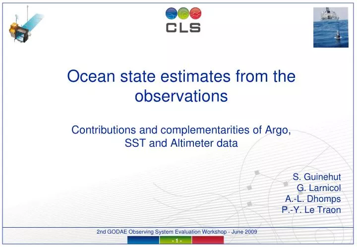
Ocean state estimates from the observations Contributions and complementarities of Argo, SST and Altimeter data. S. Guinehut G. Larnicol A.-L. Dhomps P.-Y. Le Traon. Introduction.

E N D
Ocean state estimates from the observations Contributions and complementarities of Argo, SST and Altimeter data S. Guinehut G. Larnicol A.-L. Dhomps P.-Y. Le Traon
Introduction • Producing comprehensive and regular information about the ocean the priority of operational oceanography and climate studies • Our approach : • Consists in estimating 3D-thermohaline fields using ONLY observations • Represents an alternative to the one developed by forecasting centers – based on model/assimilation techniques • Observed component of the Global MyOcean Monitoring and Forecasting Center leads by Mercator • Rely on the combine use of observations and statistical methods (linear regression + mapping) • Previous studies have shown the capability of such approach : • In producing reliable ocean state estimates (Guinehut et al., 2004; Larnicol et al., 2006) • In analyzing the contribution and complementarities of the different observing systems (in-situ vs. remote-sensing) (1st GODAE OSE Workshop, 2007) • Method revisited here : • How Argo observations help us to improve the accuracy of our ocean state estimates • Contribution/complementarities of the different observing systems
The principle The observations The method The products 3D Ocean State [T,S,U,V] daily, weekly [0-1500m] [1/3°] Altimeter, SST, winds Guinehut et al., 2004 Guinehut et al., 2006 Larnicol et al., 2006 Rio et al., 2009 Validation of model simulations Analysis of the ocean variability OSE / OSSE T/S profiles, surface drifters
3D - T/S products vertical projection of satellite data (SLA, SST) combination of synthetic and in-situ profiles 1 2 synthetic T(z), S(z) SLA, SST multiple linear regression 1 optimal interpolation 2 combined T(z), S(z) in-situ T(z), S(z)
The method – step 1 vertical projection of satellite data (SLA, SST) linear regression method 1 T(z) = (z).SLAsteric + (z).SST’ + Tclim (z) S(z)=’(z).SLAsteric + Sclim (z) • How Argo improves the accuracy of the synthetic estimates Old vs. New ? • Choice of [T,S] climatology : Levitus 05 to ARIVO (Ifremer) • Altimeter pre-processing: sea level # dynamic height anomalies • Barotropic/baroclinic partition: extraction of the steric part • (z), (z) local covariances computed from historical observations
3D - T/S products Old (V1)New (V2) • DUACS • Guinehut et al. (2006) • Reynolds OI-SST 1°-weekly • Levitus 05 • WOD 01 - annual • 700 m (1500 m) • Altimetry • Products • Barotropic/baroclinic partition • SST • Products • Method • Referenceclimatology • Covariances • Max depth • DUACS • Dhomps et al. (2009) • Reynolds OI-SST ¼°-daily • ARIVO • WOD 05 + Argo - seasonal • 1500 m
Barotropic / Baroclinic partition • SLAsteric = SLA. Reg-coef • Old - V1 Guinehut et al., 2006 : use 1993-2003 observations • New - V2 Dhomps et al., 2009 (to be sub) : use 2001-2007 Argo data (Coriolis) Regression coefficient between SLA and DHA (0-1500m) • Much better global coverage • More accurate estimates thanks to salinity data • Deeper estimate (1500 m vs. 700 m)
New covariances WOD 05 + ARGO WOD01 • Better coverage and continuity in the Southern Ocean • With increased values • More accurate estimates thanks to salinity data • Deeper estimate (1500 m vs. 700 m)
Validation of step-1 • Results over the year 2007 • 3D – T/S synthetic fields : weekly, [0-1500m], 1/3° grid • Validation by comparison with in-situ profiles Repartition of the in-situ T/S profiles valid up to 1500 m
Levitus 05 Arivo Old-V1 New-v2 Validation of step-1 / temperature Mean difference (°C) RMS difference (°C) Rms difference (% variance) • Big impact of the climatology – reduction of the bias at all depths • Improvement at the surface higher resolution SST • Improvement in the mixed layer seasonal covariances • Improvement at depth more precise covariances (Argo T/S) • Improvements : • 20 % in the surf layers • Up to 40 % at depth
Validation of step-1 / temperature / impact of SST OI-SST 1° Section at 35°N T at 30m SST OI-SST ¼° Section at 35°N T at 30m SST
Levitus 05 Arivo Old-V1 New-v2 Validation of step-1 / salinity Mean difference (psu) Rms difference (psu) Rms difference (% variance) • Improvement similar than for temperature • Much more difficult to infer salinity at depth from surface measurements • Improvements : • 35 % at all depths
Summary – step 1 results • Using simple statistical techniques, about 50 to 60 % of the variance of the T field can be deduced from SLA+SST • More difficult to reconstruct S at depth from SLA and statistics – 40 to 50 % of the variance of the S field nevertheless reconstructed • Indirectly, Argo observations have helped a lot to improve the accuracy of the method • Deeper estimates (1500 m vs. 700 m) • More precise globally (Southern Oceans) • 20 to 40 % at depth for the T field • 35 % for the S field
The method – step 2 combination of synthetic and in-situ profiles optimal interpolation method 2 Not change much yet (perspectives: correlation scales, error …) How it works : ex. T anomaly field at 100 m Synthetic T In-situ observations Combined T Argo T
Observing System Evaluation • 4 “products” : • Climatology (=Arivo) - monthly fields • Synthetic fields - weekly fields • Combined fields • Argo fields • Observing system evaluation : • Combined fields / Argo fields SLA+SST / SLA impact • Combined fields / Synthetic fields Argo impact • Argo fields / Arivo Argo impact (when no remote-sensing) • Synthetic fields / Arivo SLA+SST / SLA impact (when no Argo)
Year 2007 Levitus 05 Arivo Synth CombinedArgo Observing System Evaluation Temperature Mean difference (°C) RMS difference (°C) Rms difference (% variance) • Combined fields / Argo fields SLA+SST impact ~ 20 % • Combined fields / Synthetic fields Argo impact ~ 20 % to 30 % at depth • Argo fields / Arivo Argo impact (when no remote-sensing) ~ 30 to 40 % • Synthetic fields / Arivo SLA+SST impact (when no Argo) ~ 40 to 10 % at depth Argo important at depth
Levitus 05 Arivo Synth CombinedArgo Observing System Evaluation Temperature • Argo mandatory at depth – in the eq. zones • SLA+SST important in the Southern Oceans
! Negative values means that the errors are decreased Observing System Evaluation Temperature at 10 m SLA+SST impact (when no Argo) Argo impact (when no remote-sensing) Argo impact (when remote-sensing) SLA+SST impact (when Argo)
! Negative values means that the errors are decreased Observing System Evaluation Temperature at 300 m SLA+SST impact (when no Argo) Argo impact (when no remote-sensing) SLA+SST impact Argo impact
Year 2007 Levitus 05 Arivo Synth CombinedArgo Observing System Evaluation Salinity Mean difference (°C) RMS difference (°C) Rms difference (% variance) • Combined fields / Argo fields SLA impact ~ 10 % • Combined fields / Synthetic fields Argo impact ~ 30 % • Argo fields / Arivo Argo impact (when no remote-sensing) ~ 30 to 40 % • Synthetic fields / Arivo SLA impact (when no Argo) ~ 10 to 20 % at depth Argo mandatory for salinity
Levitus 05 Arivo Synth CombinedArgo Observing System Evaluation Temperature • Very little impact of SLA in the eq. zones • Argo mandatory everywhere
! Negative values means that the errors are decreased Observing System Evaluation Salinity at 10 m SLA impact (when no Argo) Argo impact (when no SLA) SLA impact (when Argo) Argo impact (when SLA)
! Negative values means that the errors are decreased Observing System Evaluation Salinity at 1200 m SLA impact (when no Argo) Argo impact (when no SLA) Argo impact (when SLA) SLA impact (when Argo)
Conclusion • Using simple statistical techniques, about 50 to 60 % of the variance of the T field can be deduced from SLA+SST – the use of Argo improve the estimate by 20 to 30 % • More difficult to reconstruct S at depth from SLA and statistics – 40 to 50 % of the variance of the S field nevertheless reconstructed – the use of Argo improve the estimate by 30 % • Ocean state estimate tool : • able to evaluate the impact and complementarities of the different observing systems • less expensive than the model/assimilation tools (conventional OSE/OSSE) • limitations : surface layers / temporal and spatial resolution / no interactions between the variable (T/S) • OSSE studies can also be performed using model outputs – done in the past (Guinehut et al., 2002; 2004) extended to future missions (HR altimetry, Argo design, deep floats, …) • This analysis tool can be easily implemented for routine monitoring • Plans to implement this tool in the frame of MyOcean • The metrics have to be defined • Need to better understand the limitation of this approach