Download
1 / 17
170 likes | 279 Views
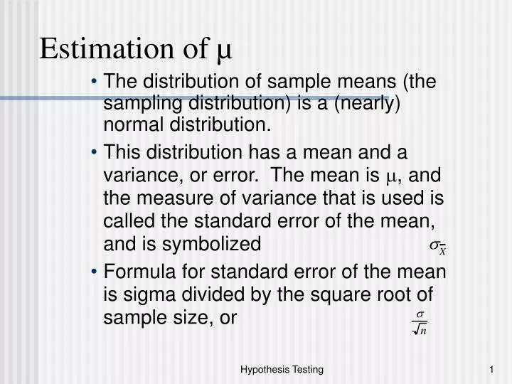
Estimation of µ. The distribution of sample means (the sampling distribution) is a (nearly) normal distribution. This distribution has a mean and a variance, or error. The mean is , and the measure of variance that is used is called the standard error of the mean, and is symbolized

E N D
Estimation of µ • The distribution of sample means (the sampling distribution) is a (nearly) normal distribution. • This distribution has a mean and a variance, or error. The mean is , and the measure of variance that is used is called the standard error of the mean, and is symbolized • Formula for standard error of the mean is sigma divided by the square root of sample size, or Hypothesis Testing
CLT • As sample size increases to equal to or greater than 10 , the sampling distribution approaches normality. This phenomenon is referred to as the Central Limit Theorem. • Definition of CLT: For any populations with mean µand standard deviation , the distribution of sample means for sample size n will approach a normal distribution with a mean of µand a standard error of s/[sq.rt(n)] as n approaches infinity. • The sampling distribution with n≥30 is normal, regardless of the shape of the original population. Hypothesis Testing
Law of Large Numbers • The law of large numbers states that the larger the sample size (n), the more probable it is that the sample mean will be close to the population mean. • Large samples are reliable, due to the lack of variability in the sampling distribution. • The estimate of the standard error of the mean: Hypothesis Testing
HYPOTHESIS TESTING • Always test Ho, the null hypothesis. • The null hypothesis states that takes on a specified value. • Always include an alternative hypothesis, H1. • The alternative hypothesis states that takes on a value other than that specified by Ho. Hypothesis Testing
Formalization • The set-ups: • Ho: µ=V, where V is some specified value • H1: µ≠V • Ho: µ=V, where V is some specified value • H1: µ<V • Ho: µ=V, where V is some specified value • H1: µ>V Hypothesis Testing
Test of the null hypothesis Hypothesis Testing
Example time • They say everything is bigger in Texas. (pause for hilarious laughter from the class.) • M, the naïve lad from the Savannah, is told that the mosquitoes are so large that they can put dents in car fenders. Although naïve, M is not stupid, so he knows hyperbole when he hears it. The Texans tell M that the average Texas “skeeter” weighs in at a remarkable 3000 mg. M is both impressed and terrified, and given his scientific tendencies, decides to test this claim. So, he goes around the state, obtaining a random sampling of 225 of the critters. One thing that M does know for certain from reading his entomology books is that the population standard deviation for the weight of Texas mosquitoes is 75mg. Hypothesis Testing
Example (cont.) • M’s sample yields an average weight of 3020mg. So, the question is, do we reject or fail to reject the claim made by these crazy Texans? • Ho: µ=3000mg • H1: µ≠3000mg Hypothesis Testing
cont. • Ho: µ=3000mg • H1: µ≠3000mg • 75mg; n=225; =3020mg • =75/ = 5 • Remember ? Hypothesis Testing
Test of the null hypothesis (cont.) • Reject the null hypothesis when z indicates that the sample mean is an extreme value. How extreme? When the probability of sampling a mean as extreme or more extreme than the sample mean occurs 5% of the time or less. • When to reject the null hypothesis? If your z-score indicates a sample mean that occurs with a frequency of 5% or less. Hypothesis Testing
Decision Rule • The z-score that we calculate is referred to as zcalc. The z-score based on the alpha level (what the hell is that?) is referred to as zcrit. • The decision rule is straightforward. When abs. value of zcalc equals or exceeds abs. value of zcrit,, reject the null hypothesis. When zcalc does not exceed, conclude that your results are inconclusive --you “fail to reject” the null hypothesis. Hypothesis Testing
Significance levels and probability values • This 5% value is called the significance level or level. • Significance (or level): The probability level that must be equaled or exceeded in order to reject the null. Usually, .05; sometimes .01 • p-value: Probability of observing a mean as extreme or more extreme, assuming a true null hypothesis • e.g., If a sample mean has an associated p-value of .20, then assuming Ho to be true, the likelihood of sampling a mean this extreme (or more extreme) is .20 (or 20%) • More about p-values. • Let’s relate p-values to the “big picture” (normal curve). Hypothesis Testing
continued • Another way of saying this is that 20% of the time, you will draw samples with means that are this extreme (far from the mean specified by Ho) or more extreme. Hypothesis Testing
Variations on this example • We can change the sample mean (make it larger or smaller). • This will affect the p-value • We can alter the sample size (again, increasing or decreasing it). • This, too, will affect the p-value by affecting the standard error of the mean. • We can alter our claim (Change the value of the null hypothesis). • This will also affect the p-value! Hypothesis Testing
One- vs. two-tailed hypothesis tests • When the alternative hypothesis includes a ">" or "<", one-tailed test (because the focus is on only one tail of the distribution.) • When the alternative hypothesis includes a "≠", two-tailed test (because both tails are in play.) • All things being equal, harder to reject the null hypothesis using a two-tailed test (because z-crit is larger than it is under one-tailed conditions). Hypothesis Testing
A few examples • Crazy Johansen claims to have read that the average Odessan loves football so much that each residents spends an average of 26 hours/week talking about football. You send your crack team out to west Texas to investigate. After spying on a random sample of 36 residents, you find the following: • Mean: 38 hrs/week • : 10 hrs z = (38 - 26)/10/sqrt(36) Hypothesis Testing
A few examples • Larry the Loon claims that the average Austin house is constructed with 1,035 nails hammered into the wood framing. You and your crack team decide to investigate. Under the cover of darkness, you disassemble 16 houses, and after hiring a good bail bondsman to free your crack team, you report the following: • Mean: 1,300 nails/house • : 400 nails z = (1,300 - 1,035)/400/sqrt(16) Hypothesis Testing