Linear Filters in Image Processing: Basics and Applications

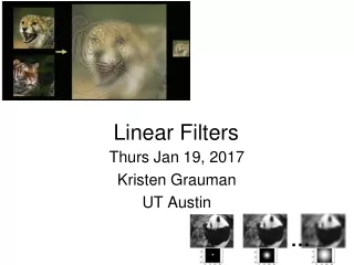
1. Linear Filters Thurs Jan 19, 2017 Kristen Grauman UT Austin …

2. Announcements • Piazza for assignment questions • A0 due Friday Jan 27. Submit on Canvas.

3. Course homepage • http://vision.cs.utexas.edu/378h-spring2017/

5. Plan for today • Image noise • Linear filters • Examples: smoothing filters • Convolution / correlation

6. Images as matrices Result of averaging 100 similar snapshots Little Leaguer Kids with Santa The Graduate Newlyweds From: 100 Special Moments, by Jason Salavon (2004) http://salavon.com/SpecialMoments/SpecialMoments.shtml

7. Image Formation Slide credit: Derek Hoiem

8. Digital camera A digital camera replaces film with a sensor array • Each cell in the array is light-sensitive diode that converts photons to electrons • http://electronics.howstuffworks.com/digital-camera.htm Slide by Steve Seitz

9. Digital images Slide credit: Derek Hoiem

10. Digital images • Sample the 2D space on a regular grid • Quantize each sample (round to nearest integer) • Image thus represented as a matrix of integer values. 2D 1D Adapted from S. Seitz

11. Digital color images

12. Digital color images Color images, RGB color space B R G

13. Images in Matlab • Images represented as a matrix • Suppose we have a NxM RGB image called “im” • im(1,1,1) = top-left pixel value in R-channel • im(y, x, b) = y pixels down, x pixels to right in the bth channel • im(N, M, 3) = bottom-right pixel in B-channel • imread(filename) returns a uint8 image (values 0 to 255) • Convert to double format (values 0 to 1) with im2double column row R G B Slide credit: Derek Hoiem

14. Main idea: image filtering • Compute a function of the local neighborhood at each pixel in the image • Function specified by a “filter” or mask saying how to combine values from neighbors. • Uses of filtering: • Enhance an image (denoise, resize, etc) • Extract information (texture, edges, etc) • Detect patterns (template matching) Adapted from Derek Hoiem

15. Motivation: noise reduction • Even multiple images of the same static scene will not be identical.

16. Common types of noise • Salt and pepper noise: random occurrences of black and white pixels • Impulse noise: random occurrences of white pixels • Gaussian noise: variations in intensity drawn from a Gaussian normal distribution Source: S. Seitz

17. Gaussian noise >> noise = randn(size(im)).*sigma; >> output = im + noise; What is impact of the sigma? Fig: M. Hebert

18. Effect of sigma on Gaussian noise: Image shows the noise values themselves.

19. Effect of sigma on Gaussian noise: Image shows the noise values themselves.

20. Effect of sigma on Gaussian noise: This shows the noise values added to the raw intensities of an image. sigma=1

21. Effect of sigma on Gaussian noise: Image shows the noise values themselves.

22. Effect of sigma on Gaussian noise This shows the noise values added to the raw intensities of an image. sigma=16

23. Motivation: noise reduction • Even multiple images of the same static scene will not be identical. • How could we reduce the noise, i.e., give an estimate of the true intensities? • What if there’s only one image?

24. First attempt at a solution • Let’s replace each pixel with an average of all the values in its neighborhood • Assumptions: • Expect pixels to be like their neighbors • Expect noise processes to be independent from pixel to pixel

25. First attempt at a solution • Let’s replace each pixel with an average of all the values in its neighborhood • Moving average in 1D: • Source: S. Marschner

26. Weighted Moving Average • Can add weights to our moving average • Weights [1, 1, 1, 1, 1] / 5 • Source: S. Marschner

27. Weighted Moving Average • Non-uniform weights [1, 4, 6, 4, 1] / 16 • Source: S. Marschner

28. Moving Average In 2D • Source: S. Seitz

29. Moving Average In 2D • Source: S. Seitz

30. Moving Average In 2D • Source: S. Seitz

31. Moving Average In 2D • Source: S. Seitz

32. Moving Average In 2D • Source: S. Seitz

33. Moving Average In 2D • Source: S. Seitz

34. Correlation filtering Say the averaging window size is 2k+1 x 2k+1: Attribute uniform weight to each pixel Loop over all pixels in neighborhood around image pixel F[i,j] Now generalize to allow different weights depending on neighboring pixel’s relative position: Non-uniform weights

35. Correlation filtering This is called cross-correlation, denoted Filtering an image: replace each pixel with a linear combination of its neighbors. The filter “kernel” or “mask” H[u,v] is the prescription for the weights in the linear combination.

36. 1 1 1 1 1 1 1 1 1 Averaging filter • What values belong in the kernel H for the moving average example? ? “box filter”

37. Smoothing by averaging depicts box filter: white = high value, black = low value filtered original What if the filter size was 5 x 5 instead of 3 x 3?

38. Boundary issues • What is the size of the output? • MATLAB: output size / “shape” options • shape = ‘full’: output size is sum of sizes of f and g • shape = ‘same’: output size is same as f • shape = ‘valid’: output size is difference of sizes of f and g • full • same • valid • g • g • g • g • f • f • f • g • g • g • g • g • g • g • g • Source: S. Lazebnik

39. Boundary issues • What about near the edge? • the filter window falls off the edge of the image • need to extrapolate • methods: • clip filter (black) • wrap around • copy edge • reflect across edge • Source: S. Marschner

40. Boundary issues • What about near the edge? • the filter window falls off the edge of the image • need to extrapolate • methods (MATLAB): • clip filter (black): imfilter(f, g, 0) • wrap around: imfilter(f, g, ‘circular’) • copy edge: imfilter(f, g, ‘replicate’) • reflect across edge: imfilter(f, g, ‘symmetric’) • Source: S. Marschner

41. Gaussian filter • What if we want nearest neighboring pixels to have the most influence on the output? • Removes high-frequency components from the image (“low-pass filter”). This kernel is an approximation of a 2d Gaussian function: Source: S. Seitz

42. Smoothing with a Gaussian

43. Gaussian filters • What parameters matter here? • Size of kernel or mask • Note, Gaussian function has infinite support, but discrete filters use finite kernels σ = 5 with 10 x 10 kernel σ = 5 with 30 x 30 kernel

44. Gaussian filters • What parameters matter here? • Variance of Gaussian: determines extent of smoothing σ = 2 with 30 x 30 kernel σ = 5 with 30 x 30 kernel

45. Matlab >> hsize = 10; >> sigma = 5; >> h = fspecial(‘gaussian’ hsize, sigma); >> mesh(h); >> imagesc(h); >> outim = imfilter(im, h); % correlation >> imshow(outim); outim

46. Smoothing with a Gaussian Parameter σ is the “scale” / “width” / “spread” of the Gaussian kernel, and controls the amount of smoothing. for sigma=1:3:10 h = fspecial('gaussian‘, fsize, sigma); out = imfilter(im, h); imshow(out); pause; end …

47. Keeping the two Gaussians in play straight… More noise  Wider smoothing kernel 

48. Properties of smoothing filters • Smoothing • Values positive • Sum to 1  constant regions same as input • Amount of smoothing proportional to mask size • Remove “high-frequency” components; “low-pass” filter

49. 1 0 0 0 0 1 0 0 0 0 0 1 1 0 0 0 2 0 1 1 0 0 1 1 0 0 1 0 1 0 0 0 0 0 0 1 Predict the outputs using correlation filtering = ? = ? * * - = ? *

50. 0 • 0 • 0 • 0 • 1 • 0 • 0 • 0 • 0 Practice with linear filters • ? • Original • Source: D. Lowe