Download

1 / 18
190 likes | 510 Views
Chapter 2: Modeling Distributions of Data. Section 2.1 Describing Location in a Distribution. The Practice of Statistics, 4 th edition - For AP* STARNES, YATES, MOORE. Measuring Position: Percentiles

E N D
Chapter 2: Modeling Distributions of Data Section 2.1 Describing Location in a Distribution The Practice of Statistics, 4th edition - For AP* STARNES, YATES, MOORE
Measuring Position: Percentiles One way to describe the location of a value in a distribution is to tell what percent of observations are less than it. Definition: The pth percentile of a distribution is the value with p percent of the observations less than it. Example 1: Jenny earned a score of 86 on her test. How did she perform relative to the rest of the class? 6 7 7 2334 7 5777899 8 00123334 8 569 9 03 6 7 7 2334 7 5777899 8 00123334 8 569 9 03 Her score was greater than 21 of the 25 observations. Since 21 of the 25, or 84%, of the scores are below hers, Jenny is at the 84th percentile in the class’s test score distribution.
Cumulative Relative Frequency Graphs A cumulative relative frequency graph (or ogive) displays the cumulative relative frequency of each class of a frequency distribution.
Interpreting Cumulative Relative Frequency Graphs Example 2: Use the graph below to answer the following questions. a) Was Barack Obama, who was inaugurated at age 47, unusually young? b) Estimate and interpret the 65th percentile of the distribution. 65 11 58 47
Measuring Position: z-Scores A z-score tells us how many standard deviations from the mean an observation falls, and in what direction. Definition: If x is an observation from a distribution that has known mean and standard deviation, the standardized value of x is: A standardized value is often called a z-score. Example 3: Jenny earned a score of 86 on her test. The class mean is 80 and the standard deviation is 6.07. What is her standardized score? That is, Jenny’s test score is about one standard deviation above the mean score of the class.
We can use z-scores to compare the position of individuals in different distributions. Using z-scores for Comparison Example 4: Jenny earned a score of 86 on her statistics test. The class mean was 80 and the standard deviation was 6.07. She earned a score of 82 on her chemistry test. The chemistry scores had a fairly symmetric distribution with a mean 76 and standard deviation of 4. On which test did Jenny perform better relative to the rest of her class?
Transforming converts the original observations from the original units of measurements to another scale. Transformations can affect the shape, center, and spread of a distribution. Transforming Data Effect of Adding (or Subracting) a Constant • Adding the same number a (either positive, zero, or negative) to each observation: • adds a to measures of center and location (mean, median, quartiles, percentiles), but • Does not change the shape of the distribution or measures of spread (range, IQR, standard deviation).
Example 5: To find the standardized score (z-score) for an individual observation, we transform this data value by subtracting the mean and dividing by the standard deviation. Transforming converts the observation from the original units of measurement (inches, for example) to a standardized scale. What effect do these kinds of transformations—adding or subtracting; multiplying or dividing—have on the shape, center, and spread of the entire distribution? Let’s investigate using an interesting data set from “down under.” Soon after the metric system was introduced in Australia, a group of students was asked to guess the width of their classroom to the nearest meter. Here are their guesses in order from lowest to highest: 8 9 10 10 10 10 10 10 11 11 11 11 12 12 13 13 13 14 14 14 15 15 15 15 15 15 15 15 16 16 16 17 17 17 17 18 18 20 22 25 27 35 38 40 Let’s talk about shape, center, spread, and outliers.
Shape:The distribution is skewed to the right. You can also say that it is bimodal with peaks at 10 and 15. Center:The median guess was 15 meters and the mean guess was about 16 meters. Due to the clear skewness and potential outliers, the median is a better choice for summarizing the “typical” guess. Spread: Since Q1 = 11, about 25% of the students estimated the width of the room at 11 meters or less. The 75th percentile of the distribution is at about Q3 = 17. The IQR of 6 meters describes the spread of the middle 50% of students’ guesses. The standard deviation tells us that the average distance of students’ guesses from the mean was about 7 meters. Since sx is not resistant to extreme values, we prefer the five-number summary and IQR to describe the variability of this distribution. Outliers: By the 1.5 × IQR rule, values greater than 17 + 9 = 26 meters or less than 11 − 9 = 2 meters are identified as outliers. So the four highest guesses− 27, 35, 38, and 40 meters —are outliers.
Effect of subtracting a constant The figure above shows dot plots of students’ original guesses and their errors on the same scale. We can see that the original distribution of guesses has been shifted to the left. By how much? Since the peak at 15 meters in the original graph is located at 2 meters in the error distribution, the original data values have been translated 13 units to the left. That should make sense: we calculated the errors by subtracting the actual room width, 13 meters, from each student’s guess.
From the figure on the previous slide, it seems clear that subtracting 13 from each observation did not affect the shape or spread of the distribution. But this transformation appears to have decreased the center of the distribution by 13 meters. The summary statistics in the table below confirm our beliefs.
Effect of Multiplying (or Dividing) by a Constant • Multiplying (or dividing) each observation by the same number b (positive, negative, or zero): • multiplies (divides) measures of center and location by b • multiplies (divides) measures of spread by |b|, but • does not change the shape of the distribution
Example 6: During the winter months, the temperatures at the Starnes’s Colorado cabin can stay well below freezing (32°F or 0°C) for weeks at a time. To prevent the pipes from freezing, Mrs. Starnes sets the thermostat at 50°F. She also buys a digital thermometer that records the indoor temperature each night at midnight. Unfortunately, the thermometer is programmed to measure the temperature in degrees Celsius. A dotplot and numerical summaries of the midnight temperature readings for a 30-day period are shown below. Use the fact that ˚F = (9/5)(˚C) + 32 to help you answer the following questions. a) Find the mean temperature in degrees Fahrenheit. Does the thermostat setting seem accurate? The thermostat doesn’t seem to be very accurate. It is set at 50°F, but the mean temperature over the 30-day period is about 47°F.
b) Calculate the standard deviation of the temperature readings in degrees Fahrenheit. Interpret this value in context. This means that the average distance of the temperature readings from the mean is about 4°F. That’s a lot of variation! c) The 90th percentile of the temperature readings was 11°C. What is the 90th percentile temperature in degrees Fahrenheit?
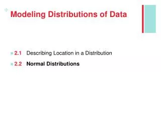
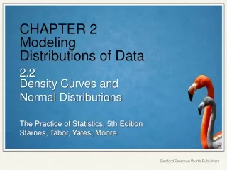
Density Curves In Chapter 1, we developed a kit of graphical and numerical tools for describing distributions. Now, we’ll add one more step to the strategy. Exploring Quantitative Data *Always plot your data: make a graph. *Look for the overall pattern (shape, center, and spread) and for striking departures such as outliers. *Calculate a numerical summary to briefly describe center and spread. *Sometimes the overall pattern of a large number of observations is so regular that we can describe it by a smooth curve.
Definition: • A density curve is a curve that • *is always on or above the horizontal axis, and • *has area exactly 1 underneath it. • A density curve describes the overall pattern of a distribution. The area under the curve and above any interval of values on the horizontal axis is the proportion of all observations that fall in that interval. The overall pattern of this histogram of the scores of all 947 seventh-grade students in Gary, Indiana, on the vocabulary part of the Iowa Test of Basic Skills (ITBS) can be described by a smooth curve drawn through the tops of the bars.
Distinguishing the Median and Mean of a Density Curve The median of a density curve is the equal-areas point, the point that divides the area under the curve in half. The mean of a density curve is the balance point, at which the curve would balance if made of solid material. The median and the mean are the same for a symmetric density curve. They both lie at the center of the curve. The mean of a skewed curve is pulled away from the median in the direction of the long tail.
1. Explain why this is a legitimate density curve. The curve is positive everywhere and it has total area of 1.0. 2. About what proportion of observations lie between 7 and 8? About 12% of the observations lie between 7 and 8. 3.Mark the approximate location of the mean and the median. A = median B = mean 4.Explain why the mean and median have the relationship that they do in this case. The mean is less than the median in this case because the distribution is skewed to the left and the mean is not resistant so it will be affected by the lower values.