Download

1 / 27
270 likes | 473 Views
Lower-branch travelling waves and transition to turbulence in pipe flow. Dr Yohann Duguet , Linné Flow Centre, KTH, Stockholm, Sweden, formerly : School of Mathematics, University of Bristol, UK. Overview. Laminar/turbulent boundary in pipe flow

E N D
Lower-branch travelling waves and transition to turbulence in pipe flow Dr Yohann Duguet, Linné Flow Centre, KTH, Stockholm, Sweden, formerly : School of Mathematics, University of Bristol, UK
Overview • Laminar/turbulent boundary in pipe flow • Identification of finite-amplitude solutions along edge trajectories • Generalisation to longer computational domains • Implications on the transition scenario
Colleagues, University of Bristol, UK • Rich Kerswell • Ashley Willis • Chris Pringle
Cylindrical pipe flow U : bulk velocity s D z L Driving force : fixed mass flux The laminar flow is stable to infinitesimal disturbances
Incompressible N.S. equations Numerical DNS code developed by A.P. Willis Additional boundary conditions for numerics :
Parameters Re = 2875, L ~ 5D, m0=1 (Schneider et. Al., 2007) Numerical resolution (30,15,15) O(105) d. o. f. Initial conditions for the bisection method Axial average
Function ri(t) rmin(t)
Starting guesses A B rmin =O(10-1)
Convergence using a Newton-Krylov algorithm rmin = O(10-11)
The skeleton of the dynamics on the edge Recurrent visits to a Travelling Wave solution …
A solution with only at least two unstable eigenvectors remains a saddle point on the laminar-turbulent boundary Eu Es Eu
A solution with only one unstable eigenvector should be a local attractor on the laminar-turbulent boundary Eu Es Es
Imposing symmetries can simplify the dynamics and show new solutions L ~ 2.5D, Re=2400, m0=2
Local attractors on the edge C3 (Duguet et. al., 2008, JFM 2008) 2b_1.25 (Kerswell & Tutty, 2007)
TURBULENCE B A C LAMINAR FLOW
Longer periodic domains 2.5D model of Willis : L = 50D, (35, 256, 2, m0=3) generate edge trajectory
Dynamical interpretation of slugs ? Extended turbulence « Slug » trajectory? localised TW relaminarising trajectory
Conclusions • The laminar-turbulent boundary seems to be structured around a network of exact solutions • Method to identify the most relevant exact coherent states in subcritical systems : the TWs visited near criticality • Symmetry subspaces help to identify more new solutions (see Chris Pringle’s talk) • Method seems applicable to tackle transition in real flows (implying localised structures)