SIFT: Scale-Invariant Feature Transform in Object Recognition & Robot Localization
420 likes | 803 Views
Discover the Scale-Invariant Feature Transform (SIFT) method by David Lowe for object recognition and robot localization. Learn how SIFT features are used in mosaicking different images and stitching them together. The SIFT algorithm involves detection and description stages, using distinctive image features for scale-rotation invariant applications. Recognize the importance of scale invariance in feature detection, keypoint localization, and descriptor construction. Explore feature matching techniques, approximate nearest neighbor search, and its applications in 3D object recognition, pose estimation, and model verification. Understand how SIFT aids in solving for pose under occlusion and provides illumination invariance in robot localization tasks.

SIFT: Scale-Invariant Feature Transform in Object Recognition & Robot Localization
E N D
Presentation Transcript
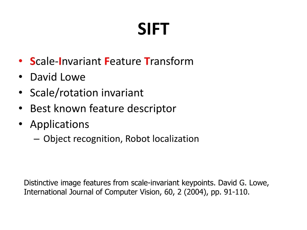
SIFT • Scale-Invariant Feature Transform • David Lowe • Scale/rotation invariant • Best known feature descriptor • Applications • Object recognition, Robot localization Distinctiveimagefeaturesfromscale-invariant keypoints.DavidG.Lowe,InternationalJournalof ComputerVision,60,2(2004),pp.91-110.
Feature detectors should be invariant or at least robust to affine changes translation rotation scale change
Example I: mosaickingUsing SIFT features we match the different images
Using those matches we estimate the homography relating the two images
SIFT Algorithm • Detection • Detect points that can be repeatably selected under location/scale change • Description • Assign orientation to detected feature points • Construct a descriptor for image patch around each feature point • Matching
ScaleInvariantDetection • Considerregionsofdifferentsize • Selectregionstosubtendthesamecontent
ScaleInvariantdetection • Howtochoosethesizeoftheregionindependently CS 685l
ScaleInvariantdetection • Sharplocalintensitychangesaregoodfunctionsfor identifyingrelativescaleoftheregion • ResponseofLaplacianofGaussians(LoG)atapoint CS 685l
1. Feature detection This is the stage where the interest points, which are called keypoints in the SIFT framework, are detected. For this, the image is convolved with Gaussian filters at different scales, and then the difference of successive Gaussian-blurred images are taken. Keypoints are then taken as maxima/minima of the Difference of Gaussians(DoG) that occur at multiple scales. This is done by comparing each pixel in the DoG images to its eight neighbors at the same scale and nine corresponding neighboring pixels in each of the neighboring scales. If the pixel value is the maximum or minimum among all compared pixels, it is selected as a candidate keypoint.
1. Feature detection • Detailed fit using data surrounding the keypoint to localize extrema by fitting a quadratic • Sub-pixel/sub-scale interpolation using Taylor expansion • Take derivative and set to zero
1. Feature detection • Discard low-contrast/edge points • Low contrast: discard keypoints with < threshold • Edge points: high contrast in one direction, low in the other compute principal curvatures from eigenvalues of 2x2 Hessian matrix, and limit ratio r is ratio of eigenvalues. Set some threshold, like rth = 10
1. Feature detection • Example • (a) 233x189 image • (b) 832 DOG extrema • (c) 729 left after peak • value threshold • (d) 536 left after testing • ratio of principle • curvatures
2. Feature description • Create histogram of local gradient directions computed at selected scale • Assign canonical orientation at peak of smoothed histogram • Assign orientation to keypoints
2. Feature description • Construct SIFT descriptor • Create array of orientation histograms • 8 orientations x 4x4 histogram array = 128 dimensions
3. Feature matching • For each feature in A, find nearest neighbor in B A B
3. Feature matching • Nearest neighbor search too slow for large database of 128-dimensional data • Approximate nearest neighbor search: Hypothesesaregeneratedbyapproximatenearest neighbormatchingofeachfeaturetovectorsinthedatabase • SIFTusebest-bin-first(Beis&Lowe,97)modificationto k-dtreealgorithm • Useheapdatastructuretoidentifybinsinorder bytheirdistancefromquerypoint • Result: Can give speedup by factor of 1000 while finding nearest neighbor (of interest) 95% of the time
3. Feature matching • Given feature matches… • Find an object in the scene • …
3. Feature matching • Example: 3D object recognition
3. Feature matching • 3D object recognition • Assume affine transform: clusters of size >=3 • Looking for 3 matches out of 3000 that agree on same object and pose: too many outliers for RANSAC or LMS • Use Hough Transform
3. Feature matching • 3D object recognition: verify model • Discard outliers for pose solution in prev step • Perform top-down check for additional features • Evaluate probability that match is correct
3D object recognition • Training images
Planar recognition • Reliably recognized at a rotation of 60° away from the camera • Affine fit is an approximation of perspective projection • Only 3 points are needed for recognition
3. Feature matching • 3D object recognition: solve for pose • Affine transform of [x,y] to [u,v]: • Rewrite to solve for transform parameters:
3D object recognition • Only 3 keys are needed for recognition, so extra keys provide robustness • Affine model is no longer as accurate