Download

1 / 24
240 likes | 340 Views
Explore the methodology of detecting communities in a social network graph using the Girvan-Newman algorithm, involving vertex betweenness, edge scoring, and iterative partitioning techniques for finding clusters.

E N D
Social network partition Presenter: Xiaofei Cao Partick Berg
Problem Statement • Say we have a graph of nodes, representing anything you can imagine, but for our purposes let’s say it represents the population spread out across a country. Some of these nodes are closely batched together, representing a “community”, while others are further away representing a different “community”. We want to detect the communities in this graph. So how do we do this?
Some Definitions • Before we try and develop a solution to this problem, we should get a few common definitions out of the way first. • Degrees – A degree is the number of edges connected to a node. • Community – A community is a grouped together (by some similarity) set of nodes that are densely connected internally.
A Degree of C is 3 B Degree of D is 2 C D E F G H
Why find Communities? • We want to find communities to see the relations between groups and their connections to others. • We can use this to find groups of people that share particular traits easily, such as terrorist organizations (or any other social network).
How do we find Communities? • Vertex Betweenness – This is a measure of a vertex (or node’s) centrality within the graph. This quantifies the number of times a node acts as a bridge in a shortest path between two other nodes.
Use BFS to find shortest-paths • We use the BFS (Breadth First Search) Algorithm to find the shortest paths between each node and every other node. • From this we can calculate the vertex betweenness for each node.
Girvan Newman Algorithm • We can use the Girvan Newman algorithm to detect communities in the graph. • Girvan Newman takes the “Betweenness” score and extends the definition to edges. • So an edge “Betweenness” score is the number of shortest paths between a pair of nodes that runs along it. • If there are more than one shortest paths, each path is assigned a value such that all paths have equal value.
Girvan Newman Algorithm Continued We can see that by using this method of edge “betweenness” scoring that communities will have lower edge scores between nodes in their community and higher edge scores along edges that connect them to other communities. To find the community, we now remove the highest scoring edge and re-calculate the “betweenness” score for each of the affected edges.
Example The highest edge score is 6, connecting node A to node C. So we remove this edge first. A C B D
Girvan Newman Algorithm Continued • Now we continue to remove each highest score edge from the graph and recalculate until no edges remain. • The end result is a dendrogram that shows the clusters of communities in our graph.
Sequential Algorithm • Proposed by Girvan-Newman in paper: "Community structure in social and biological networks." Proceedings of the National Academy of Sciences 99.12 (2002): 7821-7826. • Complete algorithm in paper: "Finding and evaluating community structure in networks." Physical review E 69.2 (2004): 026113.
Girvan Newman algorithm • Goal: find the edge with the highest betweenness score and remove it. Continue doing that until the graph been partitioned. • Import: The graph for every iteration. (adjacency matrix) • Output: The betweenness score for every edges. (Betweenness matrix) • The algorithm can be separate into 2 parts.
Part I: Find the number of shortest path from one node to every other nodes • From top to down. • Using breadth first algorithm to generate a new view for that node. • Find the number of shortest path.
7 2 1 1 1 1 3 1 1 8 5 6 1 3 2 5 1 1 1 1 1 1 1 4 2 4 2 7 6 4 5 6 3 8 3 2 7 8 View from node 1
Part II Calculate the edges betweenness score for every iteration • From bottom to up. • Every nodes contain one score. • Every edges’ score equal to Node_score/#shortest_path*(# of shortest path to the upper layer nodes) • Sum up edges’ scores for every iteration.
Score=Node_score/#shortest_path*(# of shortest path to the upper layer nodes) 7 2 1 1 1 1 3 25/6 3 11/6 1 1 3 1 1 8 5 6 1 3 2 5 1 3/2 5/6 5/6 3/2 1/2 4/3 1/2 1 1 1 1 1 1 1 4 2 4 2 7 6 4 5 6 1/2 1/2 2/3 1/3 3 8 3 7 2 8 View from node 1
Analysis the time complex • Number of iteration in the big loop: n (number of nodes) • Time complex of finding the shortest path: O(n^2) • Time complex of calculating the betweenness score:O(n) • Adding the betweenness matrix: n^2 • Time complex is: n*(n^2+n+n^2)=O(n^3);
Parallel algorithm (Intuitively) • Assigned every processor the same adjacency matrix of the original network. • They start from different nodes. Generating views and calculating the betweenness matrix for each starting nodes. Then sum the matrix locally first. • Doing prefix sum and update the original network by remove the highest score edges.
Gn: start from node n in graph P1 P2 P3 P4 P5 P6 P7 P8 G1,G2,G3 G4,G5,G6 G7,G8,G9 G10,G11,G12 G13,G14,G15 G16,G17,G18 G19,G20,G21 G22,G23,G24 Breath first algorithm V1, V2, V3 V4, V5, V6 V7, V8, V9 V10, V11, V12 V13, V14, V15 V16, V17, V18 V19, V20, V21 V22, V23, V24 Sum the between-ness score locally B1 B2 B3 B4 B5 B6 B7 B8 B1 B2 B3 B4 B5 B6 B7 B8 B1 B2 B3 B4 B5 B6 B7 B8 Parallel Prefix Sum Use B8 Value to update network B1 B2 B3 B4 B5 B6 B7 B8 B1 B2 B3 B4 B5 B6 B7 B8
Analysis of time complex • Number of iteration: n/p; • Find the number of shortest path: O(n^2); • Find the betweenness score: O(n); • Adding betweenness score locally: O(n^2); • Adding betweenness score globally(prefix sum): O(n^2*log(p)) • Time complex: n/p*(n^2+n+n^2)+n^2*log(p) =n^2(n/p+log(p));
Continue • Speed up: n/(n/p+log(P)) • When n=p*log(p); speed up = p; It is cost optimal.