Download
1 / 29
290 likes | 380 Views
Week 7: Carbon Cycle. CO 2 Fluxes into and out of the ATMO CO 2 time series: it’s going up ~0.5%/yr NPP, Rh, NEP, NBP Terrestrial Budgets Oceanic Budgets. www.geog.ouc.bc.ca/physgeog/contents/9r.html. Budgeting and time constants (box model):.

E N D
Week 7: Carbon Cycle • CO2 Fluxes into and out of the ATMO • CO2 time series: it’s going up ~0.5%/yr • NPP, Rh, NEP, NBP • Terrestrial Budgets • Oceanic Budgets
Budgeting and time constants (box model): Thus 200 yrs is the adjustment time for equilibration of CO2
Figure 3.2: Variations in atmospheric CO2 concentration on different time-scales
The terrestrial biosphere's role in the carbon cycle Carbon dioxide from the atmosphere is utilised by plants by photosynthesis. The carbon they absorb is allocated within the plant to make up its roots, wood and leaves. Some of this carbon is then lost - either when the leaves drop, or when the plant dies - and becomes soil carbon. Microbes within the soil breakdown this carbon and release it back to the atmosphere as respiration, in the form of carbon dioxide. This is the terrestrial carbon cycle on a small scale (i.e. on the scale of individual plants). On a larger scale (i.e. across geographical regions), the distribution of vegetation is important in the carbon cycle. Different plant types store different amounts of carbon, but they grow at different speeds and favour different conditions. For example trees can store more carbon than grass (per unit area of land covered), but they take a lot longer to grow. So if a previously barren area of land becomes fertile for some reason then grasses will grow first, but trees may take over later. The local climatic conditions, and how they change over time, determine which type of plant dominates in any given location. Human activity also changes the land use, and hence the carbon stored by the biosphere - cutting down trees removes a potentially large absorber of carbon dioxide and if the wood is burnt, or left to decay, then the carbon is released back to the atmosphere. Disturbance of vegetation also affects the soil - deforestation can also lead to large amounts of carbon being lost from the soil. This has an impact on the fertility of the ground and may affect future vegetation growth in the area. Such changes in land use (predominantly in the tropical forests) accounted for the most significant part of anthropogenic carbon dioxide release during the 19th Century. It was not until about 1950 that fossil fuel emissions became significantly larger than the source from land use change. Present day emissions due to anthropogenic land use change still amount to around 1 GtC per year. www.met-office.gov.uk/research/hadleycentre/models/carbon_cycle/intro_terrest.html
How CO2 interacts with plants • Stomata are the openings in leaf surfaces • CO2, O2, H2O go in and out of the Stomata • CO2 concentration controls opening size • Increased CO2 conc can increase photosyn. • It can also limit water loss (transpiration)
www.microscopy-uk.org.uk/schools/images/stomata.html Although open stomata are essential for photosynthesis, they also expose the plant to the risk of losing water through transpiration. Some 90% of the water taken up by a plant is lost in transpiration.
Stomata Water passes out of plants through small holes in the skin of the leaf. These small holes are called stomata. Each hole is surrounded by a pair of 'guard cells'. The guard cells can change shape. They can open and close each hole. The guard cells control how much water a plant loses through its leaves. They are sensitive to conditions in the environment.
www.dundee.ac.uk/bioscience/weyers3.htm Stomata from a epidermal peel of Commelina communis CO2
Some Definitions • NPP: Net Primary Production: annual plant growth=photosynthesis-autotrophic respiration. • NEP: Net Ecosystem Production (includes soil, decay of detritis [Rh]) • NBP: Net Biome Production
Global, annual net primary production (NPP) (g C/m2/y) for the land and ocean biosphere. This calculation is from models that use satellite data to calculate the absorption of visible radiation by photosynthetic pigments in plants, algae, and cyanobacteria.The land model (CASA) and the ocean model (VGPM) are similar in their reliance on broadly observed patterns to scale photosynthesis and growth from the individual to the ecosystem level.This calculation, based on ocean data for 1978–1983 and land date for 1982–1990 produces a global NPP of 104.9 Pg C/y (104.9 x 10¹⁵ g C/y), with approximately half (46.2%) contributed by the oceans and half (53.8%) contributed by the land. These approximately equal contributions to global NPP highlight the role of both land and ocean processes in the global carbon cycle.
Increasing CO2 and Plants • C3 plants (trees, most plants of cold climes) will increase biomass for increased CO2 concentration. • C4 plants (tropical and many temperate grasses, etc.) are less sensitive to CO2 concentration changes.
Figure 3.3: Fossil fuel emissions and the rate of increase of CO2 concentration in the atmosphere. The annual atmospheric increase is the measured increase during a calendar year. The monthly atmospheric increases have been filtered to remove the seasonal cycle. Vertical arrows denote El Niño events.
The oceans role in the carbon cycle Carbon dioxide from the atmosphere dissolves in the surface waters. On entering the ocean, carbon dioxide undergoes rapid chemical reactions with the water and only a small fraction remains as carbon dioxide. The carbon dioxide and the associated chemical forms are collectively known as dissolved inorganic carbon or DIC. This chemical partitioning of DIC ('buffering') affects the air–sea transfer of carbon dioxide, as only the unreacted carbon dioxide fraction in the sea water takes part in ocean–atmosphere interaction. The dissolved inorganic carbon (DIC) is transported by ocean currents. Near the poles, cold dense waters sink towards the bottom of the ocean and subsequently spread through the ocean basins. These waters return to the surface hundreds of years later. As more carbon dioxide can dissolve in cold water than in warm, these cold dense waters sinking at high latitudes are rich in carbon and act to move large quantities of carbon from the surface to deep waters. This mechanism is known as the 'solubility pump'. As well as being transported around the ocean, dissolved inorganic carbon is also used by ocean biology. In the surface waters, drifting microscopic oceanic plants known as phytoplankton grow. As with land based plants, phytoplankton take in carbon dioxide during growth and convert it to complex organic forms. The phytoplankton are eaten by drifting oceanic animals known as zooplankton, which themselves are preyed upon by other zooplankton, fish or even whales. During these biological processes, some of the carbon taken in during growth of the phytoplankton is broken down from the organic forms of the biology back to inorganic forms (DIC). If between the carbon uptake by phytoplankton and the subsequent return of the carbon to DIC, the biological material has been transported to depth, for example by the sinking of large biologically formed particles, there is a net transfer of carbon from the surface to depth. This process is termed the 'biological pump'. The carbon can also sink as skeletal structures of the biology which is known as the 'carbonate pump'.
Figure 3.1: The global carbon cycle: storages (PgC) and fluxes (PgC/yr) estimated for the 1980s. (a) Main components of the natural cycle. The thick arrows denote the most important fluxes from the point of view of the contemporary CO2 balance of the atmosphere: gross primary production and respiration by the land biosphere, and physical air-sea exchange. These fluxes are approximately balanced each year, but imbalances can affect atmospheric CO2 concentration significantly over years to centuries. The thin arrows denote additional natural fluxes (dashed lines for fluxes of carbon as CaCO3), which are important on longer time-scales. The flux of 0.4 PgC/yr from atmospheric CO2 via plants to inert soil carbon is approximately balanced on a time-scale of several millenia by export of dissolved organic carbon (DOC) in rivers (Schlesinger, 1990).
Figure 3.8: Modelled fluxes of anthropogenic CO2 over the past century. (a) Ocean model results from OCMIP (Orr and Dutay, 1999; Orr et al., 2000); (b), (c) terrestrial model results from CCMLP (McGuire et al., 2001). Positive numbers denote fluxes to the atmosphere; negative numbers denote uptake from the atmosphere. The ocean model results appear smooth because they contain no interannual variability, being forced only by historical changes in atmospheric CO2. The results are truncated at 1990 because subsequent years were simulated using a CO2 concentration scenario rather than actual measurements, leading to a likely overestimate of uptake for the 1990s. The terrestrial model results include effects of historical CO2 concentrations, climate variations, and land-use changes based on Ramankutty and Foley (2000). The results were smoothed using a 10-year running mean to remove short-term variability. For comparison, grey boxes denote observational estimates of CO2 uptake by the ocean in panel (a) and by the land in panel (b) (from Table 3.1). Land-use change flux estimates from Houghton et al. (1999) are shown by the black line in panel (c). The grey boxes in panel (c) indicate the range of decadal average values for the land-use change flux accepted by the SRLULUCF (Bolin et al., 2000) for the 1980s and for 1990 to 1995.
Figure 3.9: Anthropogenic CO2 in the Atlantic Ocean (mmol/kg): comparison of data and models. The top left panel shows the sampling transect; the top right panel shows estimates of anthropogenic CO2 content along this transect using observations from several cruises between 1981 and 1989 (Gruber, 1998). Anthropogenic CO2 is not measured directly but is separated from the large background of oceanic carbon by an indirect method based on observations (Gruber et al., 1996). The remaining panels show simulations of anthropogenic CO2 content made with four ocean carbon models forced by the same atmospheric CO2 concentration history (Orr et al., 2000).
Figure 3.10: Projections of anthropogenic CO2 uptake by process-based models. Six dynamic global vegetation models were run with IS92a CO2 concentrations as given in the SAR: (a) CO2 only, and (b) with these CO2 concentrations plus simulated climate changes obtained from the Hadley Centre climate model with CO2 and sulphate aerosol forcing from IS92a (Cramer et al., 2000). Panel (b) also shows the envelope of the results from panel (a) (in grey). (c) Ten process-based ocean carbon models were run with the same CO2 concentrations, assuming a constant climate (Orr and Dutay, 1999; Orr et al., 2000). A further six models were used to estimate the climate change impact on ocean CO2 uptake as a proportional change from the CO2-only case. The resulting changes were imposed on the mean trajectory of the simulations shown in panel (c), shown by the black line in panel (d), yielding the remaining trajectories in panel (d). The range of model results in panel (d) thus represents only the climate change impact on CO2 uptake; the range does not include the range of representations of ocean physical transport, which is depicted in panel (c).
Figure 3.11: Projected CO2 concentrations resulting from the IS92a emissions scenario. For a strict comparison with previous work, IS92a-based projections were made with two fast carbon cycle models, Bern-CC and ISAM (see Box 3.7), based on CO2 changes only, and on CO2 changes plus land and ocean climate feedbacks. Panel (a) shows the CO2 emisisons prescribed by IS92a; the panels (b) and (c) show projected CO2 concentrations for the Bern-CC and ISAM models, respectively. Results obtained for the SAR, using earlier versions of the same models, are also shown. The model ranges for ISAM were obtained by tuning the model to approximate the range of responses to CO2 and climate shown by the models in Figure 3.10, combined with a range of climate sensitivities from 1.5 to 4.5°C rise for a doubling of CO2. This approach yields a lower bound on uncertainties in the carbon cycle and climate. The model ranges for Bern-CC were obtained by combining different bounding assumptions about the behaviour of the CO2 fertilisation effect, the response of heterotrophic respiration to temperature and the turnover time of the ocean, thus approaching an upper bound on uncertainties in the carbon cycle. The effect of varying climate sensitivity from 1.5 to 4.5°C is shown separately for Bern-CC. Both models adopted a “reference case” with mid-range behaviour of the carbon cycle and climate sensitivity of 2.5°C.
Figure 3.12: Projected CO2 concentrations resulting from six SRES scenarios. The SRES scenarios represent the outcome of different assumptions about the future course of economic development, demography and technological change (see Appendix II). Panel (a) shows CO2 emissions for the selected scenarios and panels (b) and (c) show resulting CO2 concentrations as projected by two fast carbon cycle models, Bern-CC and ISAM (see Box 3.7 and Figure 3.11). The ranges represent effects of different model parametrizations and assumptions as indicated in the text and in the caption to Figure 3.11. For each model, and each scenario the reference case is shown by a black line, the upper bound (high-CO2 parametrization) is indicated by the top of the coloured area, and the lower bound (low-CO2 parametrization) by the bottom of the coloured area or (where hidden) by a dashed coloured line.
Figure 3.13: Projected CO2 emissions leading to stabilisation of atmospheric CO2 concentrations at different final values. Panel (a) shows the assumed trajectories of CO2 concentration (WRE scenarios; Wigley et al., 1996) and panels (b) and (c) show the implied CO2 emissions, as projected with two fast carbon cycle models, Bern-CC and ISAM (see Box 3.7 and Figure 3.11). The ranges represent effects of different model parametrizations and assumptions as indicated in the text and in the caption to Figure 3.11. For each model, the upper and lower bounds (corresponding to low- and high-CO2 parametrizations, respectively) are indicated by the top and bottom of the shaded area. Alternatively, the lower bound (where hidden) is indicated by a dashed line.