Download
1 / 108
2.02k likes | 3.62k Views
R. Manna Assistant Professor Centre of Advanced Study Department of Metallurgical Engineering Institute of Technology, Banaras Hindu University Varanasi-221 005, India rmanna.met@itbhu.ac.in Tata Steel-TRAERF Faculty Fellowship Visiting Scholar

E N D
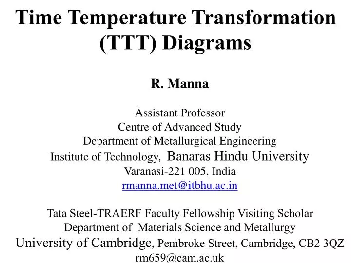
R. Manna Assistant Professor Centre of Advanced Study Department of Metallurgical Engineering Institute of Technology, Banaras Hindu University Varanasi-221 005, India rmanna.met@itbhu.ac.in Tata Steel-TRAERF Faculty Fellowship Visiting Scholar Department of Materials Science and MetallurgyUniversity of Cambridge, Pembroke Street, Cambridge, CB2 3QZrm659@cam.ac.uk Time Temperature Transformation (TTT) Diagrams
TTT diagrams TTT diagram stands for “time-temperature-transformation” diagram. It is also called isothermal transformation diagram Definition: TTT diagrams give the kinetics of isothermal transformations.
Determination of TTT diagram for eutectoid steel Davenport and Bain were the first to develop the TTT diagram of eutectoid steel. They determined pearlite and bainite portions whereas Cohen later modified and included MS and MF temperatures for martensite. There are number of methods used to determine TTT diagrams. These are salt bath (Figs. 1-2) techniques combined with metallography and hardness measurement, dilatometry (Fig. 3), electrical resistivity method, magnetic permeability, in situ diffraction techniques (X-ray, neutron), acoustic emission, thermal measurement techniques, density measurement techniques and thermodynamic predictions. Salt bath technique combined with metallography and hardness measurements is the most popular and accurate method to determine TTT diagram.
Fig. 1 : Salt bath I -austenitisation heat treatment. Fig. 2 : Bath II low-temperature salt-bath for isothermal treatment.
Fig. 3(b) : Dilatometer equipment Fig . 3(a): Sample and fixtures for dilatometric measurements
In molten salt bath technique two salt baths and one water bath are used. Salt bath I (Fig. 1) is maintained at austenetising temperature (780˚C for eutectoid steel). Salt bath II (Fig. 2) is maintained at specified temperature at which transformation is to be determined (below Ae1), typically 700-250°C for eutectoid steel. Bath III which is a cold water bath is maintained at room temperature. In bath I number of samples are austenitised at AC1+20-40°C for eutectoid and hypereutectoid steel, AC3+20-40°C for hypoeutectoid steels for about an hour. Then samples are removed from bath I and put in bath II and each one is kept for different specified period of time say t1, t2, t3, t4, tn etc. After specified times, the samples are removed and quenched in water. The microstructure of each sample is studied using metallographic techniques. The type, as well as quantity of phases, is determined on each sample.
The time taken to 1% transformation to, say pearlite or bainite is considered as transformation start time and for 99% transformation represents transformation finish. On quenching in water austenite transforms to martensite. But below 230°C it appears that transformation is time independent, only function of temperature. Therefore after keeping in bath II for a few seconds it is heated to above 230°C a few degrees so that initially transformed martensite gets tempered and gives some dark appearance in an optical microscope when etched with nital to distinguish from freshly formed martensite (white appearance in optical microscope). Followed by heating above 230°C samples are water quenched. So initially transformed martensite becomes dark in microstructure and remaining austenite transform to fresh martensite (white).
Quantity of both dark and bright etching martensites are determined. Here again the temperature of bath II at which 1% dark martensite is formed upon heating a few degrees above that temperature (230°C for plain carbon eutectoid steel) is considered as the martensite start temperature (designated MS). The temperature of bath II at which 99 % martensite is formed is called martensite finish temperature ( MF). Transformation of austenite is plotted against temperature vs time on a logarithm scale to obtain the TTT diagram. The shape of diagram looks like either S or like C. Fig. 4 shows the schematic TTT diagram for eutectoid plain carbon steel
Fig.4: Time temperature transformation (schematic) diagram for plain carbon eutectoid steel 100 T2 At T1, incubation period for pearlite=t2, Pearlite finish time =t4 Minimum incubation period t0 at the nose of the TTT diagram, T1 % of Phase 50% 0 Ae1 Austenite +pearlite Pearlite start T2 Coarse Pearlite Pearlite finish 50% Transformation Pearlite T1 t1 t2 t3 t4 Fine pearlite t5 Hardness t0 50% very fine pearlite + 50% upper bainite MS=Martensite start temperature M50=temperature for 50% martensite formation MF= martensite finish temperature Austenite+upper bainite Upper bainite Temperature Metastable austenite Bainite finish Austenite +lower bainite Bainite start Lower bainite MS, Martensite start temperature M50,50% Martensite Metastable austenite +martensite MF, Martensite finish temperature Martensite Log time
At close to Ae1 temperature, coarse pearlite forms at close to Ae1 temperature due to low driving force or nucleation rate. At higher under coolings or lower temperature finer pearlite forms. At the nose of TTT diagram very fine pearlite forms Close to the eutectoid temperature, the undercooling is low so that the driving force for the transformation is small. However, as the undercooling increases transformation accelerates until the maximum rate is obtained at the “nose” of the curve. Below this temperature the driving force for transformation continues to increase but the reaction is now impeded by slow diffusion. This is why TTT curve takes on a “C” shape with most rapid overall transformation at some intermediate temperature.
Pearlitic transformation is reconstructive. At a given temperature (say T1) the transformation starts after an incubation period (t2, at T1). Locus of t2 for different for different temperature is called transformation start line. After 50% transformation locus of that time (t3 at T1)for different temperatures is called 50% transformation line. While transformation completes that time (t4 at T1) is called transformation finish, locus of that is called transformation finish line. Therefore TTT diagram consists of different isopercentage lines of which 1%, 50% and 99% transformation lines are shown in the diagram. At high temperature while underlooling is low form coarse pearlite. At the nose temperature fine pearlite and upper bainite form simultaneously though the mechanisms of their formation are entirely different. The nose is the result of superimposition of two transformation noses that can be shown schematically as below one for pearlitic reaction other for bainitic reaction (Fig. 6). Upper bainite forms at high temperature close to the nose of TTT diagram while the lower bainite forms at lower temperature but above MS temperature.
Fig. 5(a) : The appearance of a (coarse) pearlitic microstructure under optical microscope.
Fig. 5(b): A cabbage filled with water analogy of the three-dimensional structure of a single colony of pearlite, an interpenetrating bi-crystal of ferrite and cementite.
Fig. 5(c): Optical micrograph showing colonies of pearlite . Courtesy of S. S. Babu.
Fig. 5(d): Transmission electron micrograph of extremely fine pearlite.
Fig. 5(e): Optical micrograph of extremely fine pearlite from the same sample as used to create Fig. 5(d). The individual lamellae cannot now be resolved.
Fig. 6: Time Temperature Transformation (schematic) diagram for plain carbon eutectoid steel γ=austenite α=ferrite CP=coarse pearlite P=pearlite FP=fine pearlite UB=upper bainite LB=lower bainite M=martensite MS=Martensite start temperature M50=temperature for 50% martensite formation MF= martensite finish temperature γ Ae1 γ + P Metastable γ CP P FP Hardness 50% very FP + 50% UB Temperature UB γ + UB Metastable γ LB γ + LB MS Metastable γ + M M50 MF M Log time
On cooling of metastable austenite 1% martensite forms at about 230°C. The transformation is athermal in nature. i.e. amount of transformation is time independent (characteristic amount of transformation completes in a very short time) but function of temperature alone. This temperature is called the martensite start temperature or MS. Below Ms while metastable austenite is quenched at different temperature amount of martensite increases with decreasing temperature and does not change with time. The temperature at which 99% martensite forms is called martensite finish temperature or MF. Hardness values are plotted on right Y-axis. Therefore a rough idea about mechanical properties can be guessed about the phase mix.
TTT diagram gives Nature of transformation-isothermal or athermal (time independent) or mixed Type of transformation-reconstructive, or displacive Rate of transformation Stability of phases under isothermal transformation conditions Temperature or time required to start or finish transformation Qualitative information about size scale of product Hardness of transformed products
Factors affecting TTT diagram Composition of steel- (a) carbon wt%, (b) alloying element wt% Grain size of austenite Heterogeneity of austenite Carbon wt%- As the carbon percentage increases A3 decreases, similar is the case for Ar3, i.e. austenite stabilises. So the incubation period for the austenite to pearlite increases i.e. the C curve moves to right. However after 0.77 wt%C any increase in C, Acm line goes up, i.e. austenite become less stable with respect to cementite precipitation. So transformation to pearlite becomes faster. Therefore C curve moves towards left after 0.77%C. The critical cooling rate required to prevent diffusional transformation increases with increasing or decreasing carbon percentage from 0.77%C and e for eutectoid steel is minimum. Similar is the behaviour for transformation finish time.
Pearlite formation is preceeded by ferrite in case of hypoeutectoid steel and by cementite in hypereutectoid steel. Schematic TTT diagrams for eutectoid, hypoeutectoid and hyper eutectoid steel are shown in Fig.4, Figs. 7(a)-(b) and all of them together along with schematic Fe-Fe3C metastable equilibrium are shown in Fig. 8.
Fig. 7(a) :Schematic TTT diagram for plain carbon hypoeutectoid steel Ae3 γ=austenite α=ferrite CP=coarse pearlite P=pearlite FP=fine pearlite UB=upper Bainite LB=lower Bainite M=martensite MS=Martensite start temperature M50=temperature for 50% martensite formation MF= martensite finish temperature γ+α Ae1 α+CP α+P γ+P FP t0 Hardness FP + UB UB Temperature Metastable γ LB MS M50 Metastable γ + M MF M Log time
Fig. 7(b): Schematic TTT diagram for plain carbon hypereutectoid steel Aecm γ=austenite CP=coarse pearlite P=pearlite FP=fine pearlite UB=upper Bainite LB=lower Bainite M=martensite MS=Martensite start temperature M50=temperature for 50% martensite formation γ+Fe3C Ae1 Fe3C+CP Fe3C+P γ +P Fe3C+FP t0 Hardness very FP +UB UB Temperature γ+UB Metastable γ γ+LB LB MS M50 Metastable γ + M Log time
Fig. 8: Schematic Fe-Fe3C metastable equilibrium diagram and TTT diagrams for plain carbon hypoeutectoid, eutectoid and hypereutectoid steels γ=austenite α=ferrite CP=coarse pearlite M=martensite MS=Martensite start temperature M50=temperature for 50% martensite formation MF= martensite finish temperature P=pearlite FP=fine pearlite UB=upper bainite LB=lower bainite (a) Fe-Fe3C metastable phase diagram (b) TTT diagram for hypoeutectoid steel (c ) TTT diagram for eutectoid steel (d) TTT diagram for hypereutectoid steel MS
Under isothermal conditions for various compositions proeutectoid tranformation has been summarised below (Fig. 9). In hypoeutectoid steel the observable ferrite morphologies are grain boundary allotriomorph (α)(Fig.11(a)-(d)), Widmanstätten plate (αW)(Figs. 12-16), and massive (αM) ferrite (Fig.11(f)). Grain boundary allotriomorphs form at close to Ae3 temperature or extension of Aecm line at low undercooling. Widmanstätten plates form at higher undercooling but mainly bellow Ae1. There are overlap regions where both allotriomorphs and Widmanstätten plates are observed. Equiaxed ferrite forms at lower carbon composition less than 0.29 wt%C.
Fig 9: Temperature versus composition in which various morphologies are dominant at late reaction time under isothermal condition Aecm W=Widmanstätten plate M=massive P=pearlite αub=upper bainite αlb =lower bainite Weight % carbon Austenite Ae3 Cm Ae1 0.77 0.0218 CmW αM α αW Volume % of retained austenite Pearlite Temperature Upper bainite Lower bainite MF MS Volume % of retained austenite at room temperature Mix martensite Lath martensite Plate martensite
There are overlapping regions where both equiaxed ferrite and Widmanstätten plates were observed. However at very low carbon percentage massive ferrite forms. The reconstructive and displacive mechanisms of various phase formation is shown in Fig. 10. In hypereutectoid steel both grain boundary allotriomorph and Widmanstatten plates were observed. Massive morphology was not observed in hypereutectoid steel. Grain boundary allotriomorphs were observed mainly close to Aecm or close to extension of Ae3 line but Widmanstätten plates were observed at wider temperature range than that of hypoeutectoid steel. In hypereutectoid steel there are overlapping regions of grain boundary allotrioorph and Widmanstätten cementite.
Fig. 11(a): schematic diagram of grain boundary allotriomoph ferrite, and intragranular idiomorph ferrite.
Fig.11(b): An allotriomorph of ferrite in a sample which is partially transformed into α and then quenched so that the remaining γ undergoes martensitic transformation. The allotriomorph grows rapidly along the austenite grain boundary (which is an easy diffusion path) but thickens more slowly.
Fig. 11(c): Allotriomorphic ferrite in a Fe-0.4C steel which is slowly cooled; the remaining dark-etching microstructure is fine pearlite. Note that although some α-particles might be identified as idiomorphs, they could represent sections of allotriomorphs. Micrograph courtesy of the DoITPOMS project.
Fig. 11(d): The allotriomorphs have in this slowly cooled low-carbon steel have consumed most of the austenite before the remainder transforms into a small amount of pearlite. Micrograph courtesy of the DoItPoms project. The shape of the ferrite is now determined by the impingement of particles which grow from different nucleation sites.
Fig. 11(e): An idiomorph of ferrite in a sample which is partially transformed into α and then quenched so that the remaining γ undergoes martensitic transformation. The idiomorph is crystallographically facetted.
Fig. 11(f ): Massive ferrite (αm) in Fe-0.002 wt%C alloy quenched into ice brine from 1000°C. Courtesy of T. B. Massalski
Fig. 13: The simultaneous growth of two self-accommodating plates and the consequential tent-like surface relief.
Fig. 15: Mixture of allotriomorphic ferrite, Widmanstätten ferrite and pearlite. Micrograph courtesy of DOITPOMS project.
Fig. 16 (a) Surface relief of Widmanstätten ferrite Fe-0.41C alloy, austenitised at 1200°C for 6 hrs, isothermally transformed at 700°C for 30 min and water quenced, (b) same field after light polishing and etching with nital.
For eutectoid steel banitic transformation occurs at 550 to 250°C. At higher temperature it is upper bainite and at lower temperature it is lower bainite. As C increases the austenite to ferrite decomposition becomes increasingly difficult. As bainitic transformation proceeds by the nucleation of ferrite, therefore banitic transformation range moves to higher timing and lower temperature. With increasing percentage of carbon the amount of carbide in interlath region in upper bainite increases and carbides become continuous phase. However at lower percentage of carbon they are discrete particles and amount of carbide will be less in both type of bainites. For start and finish temperatures for both types of bainites go down significantly with increasing amount of carbon (Figs. 8-9). However increasing carbon makes it easier to form lower bainite.
Fig. 18: Upper bainite; the phase between the platelets of bainitic ferrite is usually cementite.
Fig. 19: Transmission electron micrograph of a sheaf of upper bainite in a partially transformed Fe-0.43C-2Si-3Mn wt% alloy (a) optical micrograph, (b, c) bright field and corresponding dark field image of retained austenite between the sub units, (d) montage showing the structure of the sheaf.
Fig. 20 : Corresponding outline of the sub-units near the sheaf tip region of Fig. 19
Fig. 21 : AFM image showing surface relief due to individual bainite subunit which all belong to tip of sheaf. The surface relief is associated with upper bainite (without any carbide ) formed at 350°C for 2000 s in an Fe-0.24C-2.18Si-2.32Mn-1.05Ni (wt% ) alloy austenitised at 1200°C for 120 s alloy. Both austenitisation and isothermal transformation were performed in vacuum. The microstructure contains only bainitic ferrite and retained austenite. The measured shear strain is 0.26±0.02.
a b Fig. 22: Optical micrograph illustrating the sheaves of lower bainite in a partially transformed (395C), Fe-0.3C-4Cr wt% ally. The light etching matrix phase is martensite. (b) Corresponding transmission electron micrograph illustrating subunits of lower bainite.
Fig. 23 : (a) Optical micrograph showing thin and spiny lower bainite formed at 190°C for 5 hours in an Fe-1.1 wt% C steel. (b) Transmission electron micrograph showing lower bainite midrib in same steel. Courtesy of M. Oka
Fig. 24 : Schematic illustration of various other morphologies: (a) Nodular bainite, (b) columnar bainite along a prior austenite boundary, (c) grain boundary allotriomorphic bainite, (d) inverse bainite a b c d
Within the bainitic transformation temperature range, austenite of large grain size with high inclusion density promotes acicular ferrite formation under isothermal transformation condition. The morphology is shown schematically (Figs. 25-27 ) Fig. 25 : shows the morphology and nucleation site of acicular ferrite.