Download
1 / 171
1.73k likes | 1.91k Views
The Network Layer. Chapter 5. Network Layer Design Issues. Store-and-Forward Packet Switching Services Provided to the Transport Layer Implementation of Connectionless Service Implementation of Connection-Oriented Service Comparison of Virtual-Circuit and Datagram Subnets.

E N D
The Network Layer Chapter 5
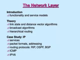
Network Layer Design Issues • Store-and-Forward Packet Switching • Services Provided to the Transport Layer • Implementation of Connectionless Service • Implementation of Connection-Oriented Service • Comparison of Virtual-Circuit and Datagram Subnets
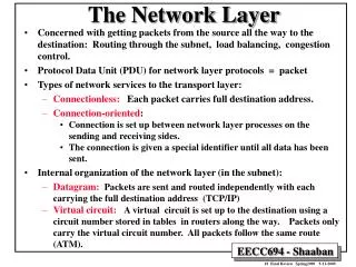
Network Layer Design Issues • Network layer provides point-to-point connectivity between any two hosts. • The network layer services have the following goals: • The services should be independent of the router technology. • The transport layer should be shielded from the number, type, and topology of the routers present. • The network addresses made available to the transport layer should use a uniform numbering plan, even across LANS and WANS. • The network layer defines the service provided by the subnet. A subnet (short for "subnetwork") is an identifiably separate part of an organization's network.
Store-and-Forward Packet Switching fig 5-1 The environment of the network layer protocols.
Functions of Network Layer • Routing – find a path from one host to another host. • Congestion control – mechanisms to prevent hosts from flooding the network. • Quality of Service (QoS) - transmission rates, error rates, and other characteristics can be measured, improved, and, to some extent, guaranteed in advance. • Internetworking provides translation between subnet using different protocols.
Services Provided to Transport Layer • The freedom in writing detailed specifications of the services to be offered to the transport layer cause battles between connection-oriented and connectionless services. • Internet community - connectionless • With 30 year experience with the Internet, the subnet is inherently unreliable. • The host should accept this fact and do error control and flow control themselves. • Telephone companies – connection-oriented • With more than 100 years’ experience, QoS is important. • QoS is important and the Internet is starting to associate with connection-oriented service.
Implementation of Services • Connectionless service • No advance setup is needed. • The packets are frequently called datagrams. • The subnet is called a datagram subnet. • The routing algorithm is the algorithm that manages the tables and makes the routing decision. • Connection-oriented service • A path from the source router to the destination router must be established before any data packets can be sent. • The connection is called a VC (virtual circuit). • The subnet is called a virtual-circuit subnet. • To distinguish packets from different hosts, replacing connection identifiers in outgoing packets is called label switching.
Implementation of Connectionless Service Routing within a diagram subnet.
Implementation of Connection-Oriented Service Routing within a virtual-circuit subnet.
Routing Algorithms • The Optimality Principle • Shortest Path Routing • Flooding • Distance Vector Routing • Link State Routing • Hierarchical Routing • Broadcast Routing • Multicast Routing • Routing for Mobile Hosts • Routing in Ad Hoc Networks
Routing Algorithms • The routing algorithm is a part of network layer software to decide which output line an incoming packet should be transmitted on. • Session routing is a route remains in force for an entire user session. • Routing algorithms should be correctness, simplicity, robustness, stability, fairness, and optimality. Conflict between fairness and optimality.
Routing Algorithms • Non-adaptive algorithms • They do not base their routing decisions on measurements or estimates of the current traffic and topology. • This procedure is sometimes called static routing. • Adaptive algorithms • They change their routing decisions to reflect changes in the topology. • This procedure is sometimes called dynamic routing.
Shortest Path Routing • If the router J is on the optimal path from the router I to the router K, then the optimal path from J to K also falls along the same route. • Proof: If there is a better router from J to K, the route from I to K can be improved. • Construct a sink tree with the destination to be root. • The goal of all routing algorithms is to discover and use the sink tree for all routers. • Since it is a tree, there is no loops. • A real network is complex. Routers and links may be down at any time.
The Optimality Principle (a) A subnet. (b) A sink tree for router B.
Shortest Path Routing • Shortest Path Routing is a static routing algorithm that just finds the shortest path. • A graph is used to represent the network. • Each node of the graph represents a router. • Each arc of the graph represents a communication link. • To choose the route between a given pair of routers, the algorithm just finds the shortest path between them on the graph. • Metric used in the shortest path. • Number of hops • Geographic distance in miles/kilometers • Transmission delay fastest path
Shortest Path Routing • Dijkstra Algorithm • Each arc (link) is labeled with a weight (link distance). • Each node is labeled with the distance from the source node along the best known path and the source node. • Initially, no paths are known, all nodes except the source are labeled as (∞, -). • All labels may be either tentative or permanent. Initially, the labels are tentative. When it is discovered to be shortest possible path, the label is made permanent and never changed thereafter..
Shortest Path Routing • An example: find the shortest path from A to D • We start out by making node A permanent indicated by a filled-in circle. • Then we examine each node adjacent to A, relabeling each one. • Scan all the tentatively labeled nodes in the whole graph and make the one with the smallest distance to A permanent. • This node becomes the new working node. Repeat the steps till the destination becomes permanent.
Shortest Path Routing The first 5 steps used in computing the shortest path from A to D. The arrows indicate the working node.
Flooding • Flooding is a static routing algorithm. • Every incoming packet is sent out on every outgoing line except the one it arrived on. • Flooding generates a large number of duplicated packets. To reduce overhead, • Use a hop counter (TTL, Time To Live), which is decremented at each hop. The packet is discarded with the counter reaches zero. • Keep track of the packets and avoid to send them out the second time in case there is a loop. • Selective flooding in which the routers send the incoming packet to only those outgoing lines in the right direction. • Flooding has tremendous reliability and always choose the shortest delay used in applications such as military, distributed database, wireless network, and a metric compared to other routing algorithm.
Flooding 5-8 top Dijkstra's algorithm to compute the shortest path through a graph.
Flooding 5-8 bottom Dijkstra's algorithm to compute the shortest path through a graph.
Distance Vector Routing • Dijkstra algorithm can find the shortest path from the source to the destination. In a real network, how the topology is obtained. • Distance Vector Routing algorithm – Dynamic routing • Each router maintains a table (vector), giving the best known distance to each destination and the outgoing line to get there. • These tables are updated by exchanging information with the neighbors. • The metric used might be the number of hops, the time delay, or the number of queued packets. • The router is assumed to know the “distance” to each of its neighbors.
Distance Vector Routing (a) A subnet. (b) Input from A, I, H, K, and the new routing table for J.
Distance Vector Routing • Distance vector works in theory but has a serious drawback in practice. • React rapidly to good news when a router comes up. • Though it finally converge to correct result, it takes long time when where is a bad news. • There are several attempts to solve the problem, but none is perfect. • Distance vector routing was used in ARPANET until 1979 when it is replaced by link state routing. • Two problems of distance vector routing: • It does not take line bandwidth into account. • It took too long to converge.
Distance Vector Routing The count-to-infinity problem.
Link State Routing • Link State Routing is a dynamic routing. • Each router must do the following: • Discover its neighbors, learn their network address. • Measure the delay or cost to each of its neighbors. • Construct a packet telling all it has just learned. • Send this packet to all other routers. • Compute the shortest path to every other router.
Learning about the Neighbors • Learning about the neighbors: When a router is booted, it first learns its immediate neighbors. • Send a HELLO packet on each point-to-point line. The router on the other end will send a reply telling who it is. • Each router has a global unique name. • If two or more routers are connected by a LAN, we can model the LAN as a node.
Learning about the Neighbors (a) Nine routers and a LAN. (b) A graph model of (a).
Measuring Line Cost • Measuring Line Cost • Send an ECHO packet, measure the round trip delay, and divide it by two. • Repeat it several items to have a better estimation. • Whether to take the load into the account? • Consider the load: start measuring delay when ECHO is queued. Choosing unloaded line results in better performance. But the load might oscillate. • Ignore the load: start measuring delay when the ECHO packet reaches the front of the queue.
Measuring Line Cost A subnet in which the East and West parts are connected by two lines.
Building Link State Packets • Build the link state packet containing: node ID, sequence number, age, a list of neighbors and the delay to the neighbor. • Building the state packet is easy. The hard part is to determine when to build them. • Periodically or event-driven (a) A subnet. (b) The link state packets for this subnet.
Distributing the Link State Packets • The trickiest part is to distribute link state packet. • Basic idea: • Use flooding to distribute the link state packets. • To keep the flood in check, each packet contains a sequence number that is increased by one for each new packet. • When the link state packet arrives, the router check if it is new. • Yes forward it to all outgoing lines except the one it arrived. • No (duplicated or with low sequence number) discard it.
Distributing the Link State Packets • Potential problems: • The sequence number wrap around use the 32-bit sequence number. It takes 137 years to wrap around. • The router crashes. Its sequence number starts again from 0, it is rejected. • The sequence number is corrupt (e.g., 65540 is received instead of 4, then packets from 5 to 65540 will be rejected.) • Use “age” to solve the problems: • The age decreases by one per second. The packet is discarded when age = 0. • Problem packets won’t last for a long time.
Distributing the Link State Packets • Each router uses a table to maintain the link state packets. • Each row is a recently received but not processed packet. • Each entry includes the source address, sequence number, age, and send/ACK flags. The packet buffer for router B in the previous slide (Fig. 5-13).
Computing Routes • Once a router has accumulated a full set of link state packets, it knows all nodes and links, thus can construct the subnet graph. • Run Dijkstra algorithm to find the shortest paths from the source to all other nodes. • For a network with n routers, each with k neighbors, the memory required in nk. • Memory and computational time may be a problem for large subnets. • But it works fine for many practical situations. • The OSPF (Open Shortest Path First) protocol is used in the Internet. • IS-IS (Intermediate System-Intermediate System) is used in some the Internet backbone (NSFNET).
Hierarchical Routing • With the increase of network/routers, it is infeasible to have an entry for each router. The hierarchical routing is required. • Divide the routers into regions. • The router only knows details to route packets to the destination within the same region. • But may not be optimal (e.g., The best route from 1A to 5C is via region 2, but since the route via region 3 is better for most nodes in region 5.
Hierarchical Routing Hierarchical routing.
Broadcast Routing • Broadcasting: send a packet to all destinations. • Distributing weather reports, stock, radio programs, etc. • Broadcast routing algorithm • Send a distinct packet to each destination (waste bandwidth) • Flooding (generate too many packets) • Multi-destination routing • The packet includes a list of destinations • The router sends the packet on an outgoing line if it is the best route for at least one of destinations (according to routing table).
Broadcast Routing • Broadcast routing algorithm • A spanning tree is a subset of the subnet that includes all the routers but contains no loops. • Copy an incoming broadcast packet onto all the spanning tree lines except the one it arrived on. • excellent use of bandwidth • But each router is required to know some spanning tree. • Reverse path forwarding: approximate spanning tree • Router check if the packet arrived on the line normally used for sending packets to the source; if so, the broadcast packet is likely following the best route, the router rebroadcast it; if no, discards it.
Broadcast Routing Reverse path forwarding. (a) A subnet. (b) a Sink tree. (c) The tree built by reverse path forwarding.
Multicast Routing • Sending a packet to a group of nodes (a subset of the nodes in the network) is called multicasting. • Multiple unicast or broadcast are too expensive • Build spanning tree • Upon receiving a packet, prune the spanning tree (cut off the routers/lines that do not lead to any member in the group) • Not scalable
Multicast Routing (a) A network. (b) A spanning tree for the leftmost router. (c) A multicast tree for group 1. (d) A multicast tree for group 2.
Routing for Mobile Hosts • All hosts are assumed to have a permanent home location (home address) that never changes. • Each area has one or more foreign agents (FA), keeping track of all mobile hosts (MH) visiting the area. • Each area has a home agent (HA), which keep track of hosts whose home is in the area but are currently visiting another area.
Routing for Mobile Hosts A WAN to which LANs, MANs, and wireless cells are attached.
Routing for Mobile Hosts • When a new host enters an area, it registers with the FA. • Each FA periodically announces its existence and address. The newly-arrived mobile host (MH) waits for one of these messages. If no message is received, it broadcasts a message and asks for FAs. • The MH sends its home address, link layer address, and some security info to the FA. • The FA contracts the HA. • The HA examines the security info and records the temporary location of the MH. • The FA gets ACK from HA, and informs MH that it has been registered.
Routing for Mobile Hosts Packet routing for mobile users.
Routing in Ad Hoc Networks Possibilities when the routers are mobile: • Military vehicles on battlefield. • No infrastructure. • A fleet of ships at sea. • All moving all the time • Emergency works at earthquake . • The infrastructure destroyed. • A gathering of people with notebook computers. • In an area lacking 802.11.
Routing in Ad Hoc Networks • A MANET (Mobile Ad Hoc Networks) is a network forming by an autonomous collection of mobile devices. • The Ad hoc On Demand Distance Vector (AODV) routing algorithm is a routing protocol designed for ad hoc mobile networks. • AODV is capable of both unicast and multicast routing. • It is an on demand algorithm, meaning that it builds routes between nodes only as desired by source nodes. • It maintains these routes as long as they are needed by the sources. • AODV forms trees which connect multicast group members. The trees are composed of the group members and the nodes needed to connect the members. • AODV uses sequence numbers to ensure the freshness of routes.
Route Discovery (a) Range of A's broadcast. (b) After B and D have received A's broadcast. (c) After C, F, and G have received A's broadcast. (d) After E, H, and I have received A's broadcast. Shaded nodes are new recipients. Arrows show possible reverse routes.