Download
1 / 51
510 likes | 636 Views
Pricing Online Banking amidst Network Effects. Baba Prasad Assistant Professor Carlson School of Management University of Minnesota, Minneapolis, MN 55455 bprasad@csom.umn.edu. Network Effects. When the value of a product is affected by how many people buy/adopt it Example: Phone System

E N D
Pricing Online Banking amidst Network Effects Baba Prasad Assistant Professor Carlson School of Management University of Minnesota, Minneapolis, MN 55455 bprasad@csom.umn.edu
Network Effects • When the value of a product is affected by how many people buy/adopt it • Example: Phone System • Types of Network Effects • Direct • Indirect • Post-purchase
Direct Network Effects • The number of users directly impacts the value of the system • Based on interaction between members of a network • E.g. Telephone service • Metcalfe’s Law: Network of size N has value O(N2)
Indirect Network Effects • Do not directly affect the value of the product • Indirect influence • Credit cards: • More adopters of the cardmore merchants accept it higher value for the card
Post-Purchase Network Effects • Mostly support related • Examples • Software user groups (LINUX Users Group) • Consumer networks
The Model • Value of a product in a market with network effects is given by: Zt is the size of the network at time t, a represents the value without network effects g represents value from network effects.
Pricing with Network Effects • Value ascribed to system by customer: Willingness to Pay (WTP) • Most optimal policy: price at WTP • Difficulty: How to determine WTP? • High collective switching costs • Leads to default standards (e.g. QWERTY; VHS, Java…)
Monopoly pricing • What happens to Coase conjecture? • Coase (1937): prices drop to marginal costs over a long period of time even in monopolistic settings
Standard Assumptions • Product purchase decision • Positive network effects • Constant parameter to represent network effect
Services and Network Effects • Assumptions in product purchase model are not valid • Not a one-time purchasing decision • Possibility of reneging and resubscribing: Market is not depleting over time
value Number of users Services and Network Effects (contd.) • Network effects can be negative • Service systems have fixed capacities • Fixed capacities deterioration in service • User notices negative network effects: • Random sampling; or word-of-mouth
Are network effects constant? • Previous discussion implies time-dependency • Thus, not really constant, but random (how many users are already on the system, when an additional user enters?) • Thus, stochastic network effects
Network Externalities in Retail Banking • Checking facility and exchange of checks • E-Checks (Kezan 1995, Stavins 1997, Ouren et al 1998) • Critical mass theory and Internet-banking users • Credit cards and indirect network effects • Introduced in 1930s, “re-introduced” in the 60s, did not take off till the mid-80s • Econometric Studies • Gowrisankaran and Stavins (1999) find strong evidence of network effects in electronic payments (ACH) • Kauffman et al have observed network effects in ATM networks
Why Electronic Banking? • Tremendous reduction in transaction costs • Coordination of Delivery Supply Chain
Cost of Transactions Across Delivery Channels Source: Jupiter Communications 1997 Home Banking Report
Coordination of Delivery Supply Chain • Electronic transactions facilitate : • Exchange of information with other banks through Electronic Clearing Houses (ECH) • Flow of information within the firm • Workflow management; process control
Banking Some Online Banking Options and Prices (March 2002) Bank
Bank Problem • Choose a price vector (P)over the two periods at the outset • Choose the optimal price vector assuming that the customer will switch in such a way as to optimize value over the two periods
Reservation Prices • Each customer indexed by h [0, 1] • Customer strategies • (0, 0): Do not choose online banking in either period • (0, 1): Choose online banking only in period 2 • (1, 0): Choose online banking in period 1 and renege in period 2 • (1, 1): Choose online banking in both periods • Let h00 (= 0), h01, h10, and h11 denote the minimal reservation prices that will allow each of these strategies
Some propositions • h11 h10 h01 0 • There exists threshold network effects gu and gl such that • when g> gu, consumers who choose online banking in period 1, do not renege in period 2, and • when g< gl , consumers who do not choose in period 1 will not do so in period 2 also.
Consumer Surplus Equations • First period V1(h, p1) = h – p1, for online banking = 0, for non-online banking • Second Period V1(h, p2, qi-1) = d(h – p2+ g qi-1) for online banking = -dCjk, for non-online banking d is the one-period discount factor (0 < d < 1)
Demand Equations • D1 = 1 – h10 and D2 = 1 – h01 • Using indifference equations between choices in the 2 periods, we arrive at: D1 = {1 – d – p1 + dp2 + d(C01 – C10)} (1 – d + dg) D2 = {(1– d + dg) (1– p2) – gp1 + dp2(1+ g) + dg(C01 – C10) – dC01 – dg2} (1–d+ dg)}
Optimal Pricing Problem P = max p1D1 + dp2D2 (p1, p2) s.t. 0 ≤ h01 ≤ h10 ≤ h11≤ 1
Optimal Prices p1* = {(1 – d) (2 – dg + d2 +2dgC10 + 2dC01) – 6d} {(d –2)2 + d2g(g-2)} p2* = {(2p1* + d(C10 +C01) – (1 – d)} {d (1 – g)}
Price behavior • Note that as g 1, p2* • Increased network effects cause higher second period benefit. • Contrast with Coase conjecture; common with other studies with positive network effects • Note also that as g increases, p1*decreases • Increased network effect leads to low introductory pricing • If d = 0, p1* = ½ and p2*
Figure 1.2. Demands at Optimal Prices in the Two Periods Demands at Optimal Prices
Intermediate Conclusions • Should banks have chosen low introductory pricing to promote online banking? • Positive switching costs lead to initial reluctance • How are issues of security and convenience perceived by consumers?
Negative word-of-mouth effects "Banking is founded on trust. We want an e-commerce service we can feel safe with, because if even one customer somewhere gets hacked - well that's bad for the customer but we suffer the impact to a greater extent because of the damage to customer trust." (Bob Lounsbury of Scotiabank, 1999) Scotia Bank was the 1998 NetCommerce Award winner in the Canada Information Productivity Association competition
Online Banking Adoption Decision • Kennikel and Kwast (1997) • 33% of respondents reported that friends and relatives who already used online banking affected decision to adopt online banking • Highest reported source of information in adoption decision • (next is financial consultants/brokers at 26.8%)
Word-of-mouth Effects • Stochastic • Can be positive or negative • Mean and variance • Affects adoption of online banking in future periods
Positive No Effect Figure 1. Transition probabilities and outcomes Negative 1- m p m 1- p - q t t + 1 q How to model W-o-M effects?
Modeling the Stochastic Network Effect • The trinomial tree can be shown to follow a Geometric Brownian motion process • Apart from “customer-talk”, expert opinion also influences demand • We model word-of-mouth effect, g, as a jump-diffusion process
Word-of-Mouth as jump-diffusion process dZ is the increment of a Wiener process, Z, with mean, mg, and s.d. sg dQ(t) is the increment of a Poisson process with mean arrival rate, l k is a draw from a normal distribution, or in other words, k ~ N(mp, sp2).
Demand function where, D(t) is demand at time t S(t) is size of network at time t p(t) is the price at time t, and g(t) is the stochastic network effect
Maximizing profit • Stochastic Optimal control • Bellman’s equation
Positive Price to Build Network Price to Penetrate Market mg Price Myopically Price to Recover Sunk Costs Negative s2 High Low Table 1. Pricing Strategy with Word-of-mouth Effects Pricing Strategy
Consumer Surplus Equations • First period V1(h, p1) = h – p1, for online banking = 0, for non-online banking • Period i, i ≥2 V1(h, p1, qi-1) = (h – p2+ g Di-1+ hiDi-1), for online banking = - Cjk, for non-online banking
Customer’s Problem • At the beginning of each period, the customer chooses a mode (online or not). The problem is to choose an optimal sequence of modes that will maximize value • To switch from mode j to mode k costs Cjk
Dynamic Program Formulation • Customer chooses to maximize value over the T periods • Consider the last period, period T: • Choose that mode that will give maximum value after discounting switching cost • Suppose customer arrives in this period in mode M VT = Max(VmT – CMm), m {Online, Non-online}
Dynamic Program Formulation (contd.) • For any period, j (0 < j) Vj-1 = Max (Vmj – C(j-1)m + dE[Vj]) E[]being the expectation, anddbeing the one-period discount factor
The Model • Value of a product exhibiting both types of network effects is given by: where Zt is the size of the network at time t, the parameter a represents the value without network effects, g represents network externality effects, and h represents word-of-mouth effects. t is the time delay for the word-of-mouth effects. For simplicity, we assume t = 1
Variation of Optimal prices with Mean of Word-of-mouth Effect 6 p2_w_o_m 4 2 p1_w_o_m p2 p1 0 -0.9 -0.8 -0.7 -0.6 -0.5 -0.4 -0.3 -0.2 -0.1 0 0.1 0.2 0.3 0.4 0.5 0.6 0.7 0.8 0.9 price --------> mean w_o_m ------> -2 -4 -6 -8
1.2 1 0.8 0.6 price_1D price _2D price_3D 0.4 0.2 h 0 1 2 3 4 5 6 7 -0.2 period Multiple Periods: Prices with Increasing Lag in Word-of-mouth Effects
Multiple Periods: Demands versus Prices with Increasing Lag in Word-of-mouth Effects • Not much variation in optimal demand • Optimal prices increase about 5% for every additional period of lag • Banks seem to be more sensitive to word-of-mouth than customers • Back to Lounsbury’s comment
Anecdotal Evidence: Bank Strategies Some Online Banking Options and Prices (March 2002) Bank