Statistical Data Analysis: Lecture 3

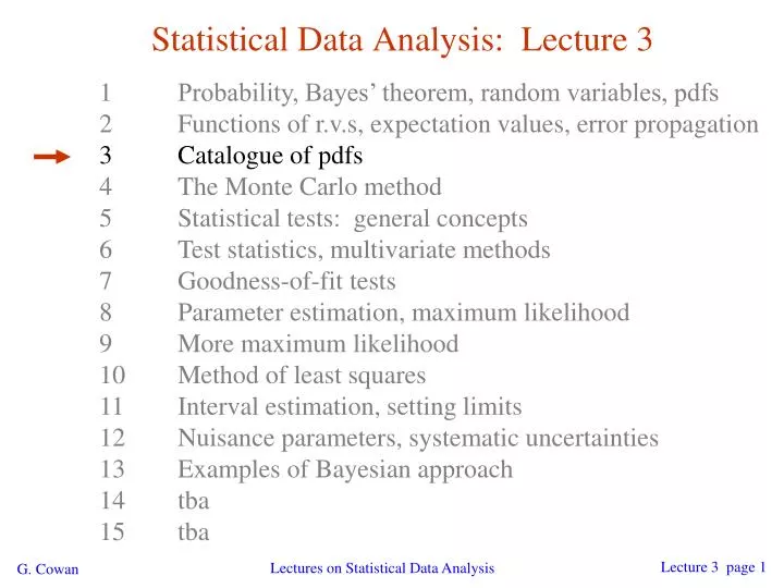
1. Statistical Data Analysis: Lecture 3 1 Probability, Bayes’ theorem, random variables, pdfs 2 Functions of r.v.s, expectation values, error propagation 3 Catalogue of pdfs 4 The Monte Carlo method 5 Statistical tests: general concepts 6 Test statistics, multivariate methods 7 Goodness-of-fit tests 8 Parameter estimation, maximum likelihood 9 More maximum likelihood 10 Method of least squares 11 Interval estimation, setting limits 12 Nuisance parameters, systematic uncertainties 13 Examples of Bayesian approach 14 tba 15 tba Lectures on Statistical Data Analysis

2. Some distributions Distribution/pdf Example use in HEP Binomial Branching ratio Multinomial Histogram with fixed N Poisson Number of events found Uniform Monte Carlo method Exponential Decay time Gaussian Measurement error Chi-square Goodness-of-fit Cauchy Mass of resonance Landau Ionization energy loss Beta Prior pdf for efficiency Gamma Sum of exponential variables Student’s t Resolution function with adjustable tails Lectures on Statistical Data Analysis

3. Binomial distribution Consider N independent experiments (Bernoulli trials): outcome of each is ‘success’ or ‘failure’, probability of success on any given trial is p. Define discrete r.v. n = number of successes (0 ≤ n ≤ N). Probability of a specific outcome (in order), e.g. ‘ssfsf’ is But order not important; there are ways (permutations) to get n successes in N trials, total probability for n is sum of probabilities for each permutation. Lectures on Statistical Data Analysis

4. Binomial distribution (2) The binomial distribution is therefore parameters random variable For the expectation value and variance we find: Lectures on Statistical Data Analysis

5. Binomial distribution (3) Binomial distribution for several values of the parameters: Example: observe N decays of W±, the number n of which are W→mn is a binomial r.v., p = branching ratio. Lectures on Statistical Data Analysis

6. Multinomial distribution Like binomial but now m outcomes instead of two, probabilities are For N trials we want the probability to obtain: n1 of outcome 1, n2 of outcome 2,  nm of outcome m. This is the multinomial distribution for Lectures on Statistical Data Analysis

7. Multinomial distribution (2) Now consider outcome i as ‘success’, all others as ‘failure’. → all ni individually binomial with parameters N, pi for all i One can also find the covariance to be represents a histogram Example: with m bins, N total entries, all entries independent. Lectures on Statistical Data Analysis

8. Poisson distribution Consider binomial n in the limit → n follows the Poisson distribution: Example: number of scattering events n with cross section s found for a fixed integrated luminosity, with Lectures on Statistical Data Analysis

9. Uniform distribution Consider a continuous r.v. x with -∞ < x < ∞ . Uniform pdf is: N.B. For any r.v. x with cumulative distribution F(x), y = F(x) is uniform in [0,1]. Example: for p0→ gg, Eg is uniform in [Emin, Emax], with Lectures on Statistical Data Analysis

10. Exponential distribution The exponential pdf for the continuous r.v. x is defined by: Example: proper decay time t of an unstable particle (t = mean lifetime) Lack of memory (unique to exponential): Lectures on Statistical Data Analysis

11. Gaussian distribution The Gaussian (normal) pdf for a continuous r.v. x is defined by: (N.B. often m, s2 denote mean, variance of any r.v., not only Gaussian.) Special case: m = 0, s2 = 1 (‘standard Gaussian’): If y ~ Gaussian with m, s2, then x = (y-m) /s follows  (x). Lectures on Statistical Data Analysis

12. Gaussian pdf and the Central Limit Theorem The Gaussian pdf is so useful because almost any random variable that is a sum of a large number of small contributions follows it. This follows from the Central Limit Theorem: For n independent r.v.s xi with finite variances si2, otherwise arbitrary pdfs, consider the sum In the limit n→ ∞, y is a Gaussian r.v. with Measurement errors are often the sum of many contributions, so frequently measured values can be treated as Gaussian r.v.s. Lectures on Statistical Data Analysis

13. Central Limit Theorem (2) The CLT can be proved using characteristic functions (Fourier transforms), see, e.g., SDA Chapter 10. For finite n, the theorem is approximately valid to the extent that the fluctuation of the sum is not dominated by one (or few) terms. Beware of measurement errors with non-Gaussian tails. Good example: velocity component vx of air molecules. OK example: total deflection due to multiple Coulomb scattering. (Rare large angle deflections give non-Gaussian tail.) Bad example: energy loss of charged particle traversing thin gas layer. (Rare collisions make up large fraction of energy loss, cf. Landau pdf.) Lectures on Statistical Data Analysis

14. Multivariate Gaussian distribution Multivariate Gaussian pdf for the vector are transpose (row) vectors, are column vectors, For n = 2 this is where r = cov[x1, x2]/(s1s2) is the correlation coefficient. Lectures on Statistical Data Analysis

15. Chi-square (c2) distribution The chi-square pdf for the continuous r.v. z (z≥ 0) is defined by n = 1, 2, ... = number of ‘degrees of freedom’ (dof) For independent Gaussian xi, i = 1, ..., n, means mi, variances si2, follows c2 pdf with n dof. Example: goodness-of-fit test variable especially in conjunction with method of least squares. Lectures on Statistical Data Analysis

16. Cauchy (Breit-Wigner) distribution The Breit-Wigner pdf for the continuous r.v. x is defined by (G = 2, x0 = 0 is the Cauchy pdf.) E[x] not well defined, V[x] →∞. x0 = mode (most probable value) G = full width at half maximum Example: mass of resonance particle, e.g. r, K*, f0, ... G = decay rate (inverse of mean lifetime) Lectures on Statistical Data Analysis

17. Landau distribution For a charged particle with b = v /c traversing a layer of matter of thickness d, the energy loss D follows the Landau pdf: D + - + - b - + - + d L. Landau, J. Phys. USSR 8 (1944) 201; see also W. Allison and J. Cobb, Ann. Rev. Nucl. Part. Sci. 30 (1980) 253. Lectures on Statistical Data Analysis

18. Landau distribution (2) Long ‘Landau tail’ →all moments ∞ Mode (most probable value) sensitive to b , →particle i.d. Lectures on Statistical Data Analysis

19. Beta distribution Often used to represent pdf of continuous r.v. nonzero only between finite limits. Lectures on Statistical Data Analysis

20. Gamma distribution Often used to represent pdf of continuous r.v. nonzero only in [0,∞]. Also e.g. sum of n exponential r.v.s or time until nth event in Poisson process ~ Gamma Lectures on Statistical Data Analysis

21. Student's t distribution n = number of degrees of freedom (not necessarily integer) n = 1 gives Cauchy, n→ ∞ gives Gaussian. Lectures on Statistical Data Analysis

22. Student's t distribution (2) If x ~ Gaussian with m = 0, s2 = 1, and z ~ c2 with n degrees of freedom, then t = x / (z/n)1/2 follows Student's t with n = n. This arises in problems where one forms the ratio of a sample mean to the sample standard deviation of Gaussian r.v.s. The Student's t provides a bell-shaped pdf with adjustable tails, ranging from those of a Gaussian, which fall off very quickly, (n → ∞, but in fact already very Gauss-like for n = two dozen), to the very long-tailed Cauchy (n = 1). Developed in 1908 by William Gosset, who worked under the pseudonym "Student" for the Guinness Brewery. Lectures on Statistical Data Analysis

23. Wrapping up lecture 3 We’ve looked at a number of important distributions: Binomial, Multinomial, Poisson, Uniform, Exponential Gaussian, Chi-square, Cauchy, Landau, Beta, Gamma, Student's t and we’ve seen the important Central Limit Theorem: explains why Gaussian r.v.s come up so often For a more complete catalogue see e.g. the handbook on statistical distributions by Christian Walck from http://www.physto.se/~walck/ Lectures on Statistical Data Analysis