ISMP Lab 新生訓練課程 Artificial Neural Networks 類神經網路
690 likes | 986 Views
National Cheng Kung University/ Walsin Lihwa Corp. 「Center for Research of E-life DIgital Technology」 成功大學/華新麗華「數位生活科技研究中心」. ISMP Lab 新生訓練課程 Artificial Neural Networks 類神經網路. 指導教授:郭耀煌 教授 碩士 班學生 : 黃盛裕 96 級 2008/7/18. Outline. Introduction Single Layer Perceptron – Perceptron

ISMP Lab 新生訓練課程 Artificial Neural Networks 類神經網路
E N D
Presentation Transcript
National Cheng Kung University/WalsinLihwa Corp. 「Center for Research of E-life DIgital Technology」 成功大學/華新麗華「數位生活科技研究中心」 ISMP Lab 新生訓練課程Artificial Neural Networks 類神經網路 指導教授:郭耀煌 教授 碩士班學生:黃盛裕 96級 2008/7/18
Outline • Introduction • Single Layer Perceptron – Perceptron • Example • Single Layer Perceptron – Adaline • Multilayer Perceptron – Back–propagation neural network • Competitive Learning - Example • Radial Basis Function (RBF) Networks • Q&A and Homework
Artificial Neural Networks (ANN) • Artificial Neural Networks • simulate human brain • approximate any nonlinear and complex functions accuracy Fig.1 Fig.2
Neural Networks vs. Computer Table 1
Biological neural networks • About 1011 neurons in human brain • About 1014~15 interconnections • Pulse-transmission frequency million times slower than electronic circuits • Face recognition • hundred million second by human • Network of artificial neuron operation speed only a few million second
Applications of ANN Pattern Recognition Fig.4 Prediction Economics Optimization VLSI Neural Networks Control Power & Energy AI Bioinformatics Communication Signal Processing Image Processing Successful apps can be found in well-constrained environment None is flexible enough to perform well outside its domain.
Challenging Problems Fig.5 • Pattern classification • Clustering/categorization • Function approximation • Prediction/forecasting • Optimization (TSP problem) • Retrieval by content • control
Brief historical review • Three periods of extensive activity • 1940s: • McCulloch and Pitts’ pioneering work • 1960s: • Rosenblatt’s perceptron convergence theorem • Minsky and Papert’s showing the limitation of a simple perceptron • 1980s: • Hopfield’s energy approach in 1982 • Werbos’ Back-propagation learning algorithm
Neuron vs. Artificial Neuron • McCulloch and Pitts propose MP neural model in 1943. • Hebb learning rule. Fig.7 Fig.6
Outline • Introduction • Single Layer Perceptron – Perceptron • Example • Single Layer Perceptron – Adaline • Multilayer Perceptron – Back–propagation neural network • Competitive Learning - Example • Radial Basis Function (RBF) Networks • Q&A and Homework
Element of Artificial Neuron Weight (Synapse) Baisθj x1 w1j x2 w2j Summation function Transfer function Output Yj wij xi …… Inputs wn-1 j xn-1 wn j xn Fig.8 The McCulloch-Pitts model (1949)
Summation function • An adder for summing the input signal, weighted by the respective synapses of the neuron. • Summation • Euclidean Distance
Transfer functions • An activation function for limiting the amplitude of the neuron of a neuron. • Threshold (step) function • Piecewise-Linear function Threshold function Yj 1 0 netj Piecewise-Linear function Yj -0.5 0.5 netj
Transfer functions Yj • Sigmoid function • Radial Basis Function Where a is the slop parameter of the sigmoid function. -0.5 0.5 netj Yj 1 Where a is the variance parameter of the radial basis function. netj -0.5 0.5
Network architectures Fig.9 A taxonomy of feed-forward and recurrent/feedback network architectures.
Network architectures • Feed-forward networks • Static: produce only one set of output value • Memory-less: independent of previous state • Recurrent (or feedback) networks • Dynamics system • Different architectures require different appropriate learning algorithm
Learning process • The ability to learn is a fundamental trait of intelligent. • Automatically learn from examples. • Instead of following a set of rules specified by human experts. • ANNs appear to learn underlying rules. • This is the major advantages over traditional expert systems.
Learning process • Learning process • Have a model of the environment • Understand how network weights are updated • Three main learning paradigms • Supervised • Unsupervised • Hybrid
Learning process • Three fundamental and practical issue of Learning theory • Capacity • Patterns • Functions • Decision boundaries • Sample complexity • The number of training samples (over-fitting) • Computational complexity • Time required (many learning algorithms have high complexity)
Learning process • Three basic types of learning rules: • Error-correction rules • Hebbian rule • If neurons on both sides of a synapse are activated synchronously and repeatedly, the synapse’s strength is selectively increased. • Competitive learning rules
Error-Correction Rules Fig.10 • The threshold function: • if v > 0 , then y = +1 • otherwise y = 0
Learning mode • On-line (Sequential) mode: • Update weights for each training data • More accurate • Require more computational time • Faster learning convergence • Off-line (Batch) mode: • Update weights after apply all training data • Less accurate • Require less computational time • Require extra storage
Error-Correction Rules • However, a single-layer perceptron can only separate linearly separable patterns as long as a monotonic activation is used. • The back-propagation learning algorithm is based on error-correction principle.
Preprocess of Neural networks • Input layers are mapping in [-1,1]. • Output layers are mapping in [0,1]
Perceptron • In 1957,A single-layer Perceptron network consists of 1 or more artificial neurons in parallel. Each neuron in the single layer provides one network output, and is usually connected to all of the external (or environmental) inputs. • Supervised • MP neuron model + Hebb learning …… …… Fig.11
Perceptron • Learning Algorithm • output • Adjust weight & bias • Energy function
Outline • Introduction • Single Layer Perceptron – Perceptron • Example • Single Layer Perceptron – Adaline • Multilayer Perceptron – Back–propagation neural network • Competitive Learning - Example • Radial Basis Function (RBF) Networks • Q&A and Homework
Perceptron Example by hand(1/11) • Use two-layer Perceptron to solve AND problem Initial parameter =0.1 =0.5 W13=1.0 W23=-1.0 X3 Fig.12 X1 X2
Perceptron Example by hand(2/11) • 1st learning cycle • Input 1st example • X1=-1, X2=-1, T=0 • net=W13•X1 +W23•X2-=-0.5, Y=0 • =T-Y=0 • W13=X1=0, W23=0, =-=0 • Input 2nd~4th example
Perceptron Example by hand(3/11) • Adjust weight & bias • W13=1, W23=-0.8, =0.5 • 2nd learning cycle
Perceptron Example by hand(4/11) • Adjust weight & bias • W13=1, W23=-0.6, =0.5 • 3rd learning cycle
Perceptron Example by hand(5/11) • Adjust weight & bias • W13=1, W23=-0.4, =0.5 • 4th learning cycle
Perceptron Example by hand(6/11) • Adjust weight & bias • W13=0.9, W23=-0.3, =0.6 • 5th learning cycle
Perceptron Example by hand(7/11) • Adjust weight & bias • W13=0.9, W23=-0.1, =0.6 • 6th learning cycle
Perceptron Example by hand(8/11) • Adjust weight & bias • W13=0.8, W23=0, =0.7 • 7th learning cycle
Perceptron Example by hand(9/11) • Adjust weight & bias • W13=0.7, W23=0.1, =0.8 • 8th learning
Perceptron Example by hand(10/11) • Adjust weight & bias • W13=0.8, W23=0.2, =0.7 • 9th learning
Perceptron Example by hand(11/11) • Adjust weight & bias • W13=0.8, W23=0.2, =0.7 • 10th learning (no change, stop learning)
Example Fig.13 input value desired output value • x1 = (1, 0, 1)T y1 = -1 • x2 = (0,−1,−1)T y2 = 1 • x3 = (−1,−0.5,−1)T y3 = 1 • the learning constant is assume to be 0.1 • The initial weight vector is w0 = (1, -1, 0)T
Step 1: • <w0, x1> = (1, -1, 0)*(1, 0, 1)T = 1 • Correction is needed since y1 = -1 ≠ sign (1) • w1 = w0 + 0.1*(-1-1)*x1 • w1 = (1, -1, 0)T – 0.2*(1, 0, 1)T = (0.8, -1, -0.2)T • Step 2: • <w1, x2> = 1.2 • y2 = 1 = sign(1.2) • w2 = w1
Step 3: • <w2, x3> = (0.8, -1, -0.2 )*(−1,−0.5,−1)T = -0.1 • Correction is needed since y3 = 1 ≠ sign (-0.1) • w3 = w2 + 0.1*(1-(-1))*x3 • w3 = (0.8, -1, -0.2 )T– 0.2*(−1,−0.5,−1)T = (0.6, -1.1, -0.4)T • Step 4: • <w3, x1> = (0.6, -1.1, -0.4)*(1, 0, 1)T = 0.2 • Correction is needed since y1 = -1 ≠ sign (0.2) • w4 = w3 + 0.1*(-1-1)*x1 • w4 = (0.6, -1.1, -0.4)T– 0.2*(1, 0, 1)T = (0.4, -1.1, -0.6)T
W6terminates the learning process. • <w6, x1> = -0.2 < 0 • <w6, x2> = 1.7 > 0 • <w6, x3> = 0.75 > 0 • Step 5: • <w4, x2> = 1.7 • y2 = 1 = sign(1.7) • w5 = w4 • Step 6: • <w5, x3> = 0.75 • y3 = 1 = sign(0.75) • w6 = w5
Adaline X1 • Architecture of Adaline • Application • Filter • communication • Learning algorithm (Least mean Square,LMS ) • Y= purelin(ΣWX-b)=W1X1+W2X2-b • W(t+1)=W(t)+2ηe(t)X(t) • b(t+1)=b(t)+2ηe(t) • e(t)=T-Y Fig.14 W1 X2 W2 Y Weight -1 b Input Layer Output Layer
Perceptron in XOR problem • XOR problem 1 1 1 ○ ○ ○ ○ × × -1 1 -1 1 -1 1 × ○ × × ○ × -1 -1 -1 OR AND XOR
Outline • Introduction • Single Layer Perceptron – Perceptron • Example • Single Layer Perceptron – Adaline • Multilayer Perceptron – Back–propagation neural network • Competitive Learning - Example • Radial Basis Function (RBF) Networks • Q&A and Homework
Multilayer Feed-Forward Networks Fig. 15 Network architectures: A taxonomy of feed-forward and recurrent/feedback network architectures.
Multilayer perceptron Xq Wqi(1) Wij(2) Wjk(L) Yk(L) x1 y1 x2 y2 xn yn Input layer Hidden layer Output layer Fig. 16 A typical three-layer feed-forward network architecture.
Multilayer perceptron • Most popular class • Which can form arbitrarily complex decision boundaries and represent any Boolean function. • Back-propagation • Let • Squared-error cost function • A geometric interpretation