Download
1 / 14
150 likes | 530 Views
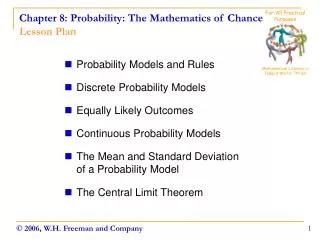
For All Practical Purposes. Chapter 8: Probability: The Mathematics of Chance Lesson Plan. Probability Models and Rules Discrete Probability Models Equally Likely Outcomes Continuous Probability Models The Mean and Standard Deviation of a Probability Model The Central Limit Theorem.

E N D
For All Practical Purposes Chapter 8: Probability: The Mathematics of ChanceLesson Plan • Probability Models and Rules • Discrete Probability Models • Equally Likely Outcomes • Continuous Probability Models • The Mean and Standard Deviation of a Probability Model • The Central Limit Theorem Mathematical Literacy in Today’s World, 7th ed. 1 © 2006, W.H. Freeman and Company
Chapter 8: Probability: The Mathematics of Chance Probability Models and Rules • Probability Theory • The mathematical description of randomness. • Companies rely on profiting from known probabilities. • Examples: Casinos know every dollar bet will yield revenue; insurance companies base their premiums on known probabilities. Randomness – A phenomenon is said to be random if individual outcomes are uncertain but the long-term pattern of many individual outcomes is predictable. Probability – For a random phenomenon, the probability of any outcome is the proportion of times the outcome would occur in a very long series of repetitions. 2
Chapter 8: Probability: The Mathematics of Chance Probability Models and Rules • Probability Model • A mathematical description of a random phenomenon consisting of two parts: a sample space S and a way of assigning probabilities to events. • Sample Space – The set of all possible outcomes. • Event – A subset of a sample space (can be an outcome or set of outcomes). • Probability Model Rolling Two Dice • Rolling two dice and summing the spots on the up faces. Probability histogram Rolling Two Dice: Sample Space and Probabilities 3
Chapter 8: Probability: The Mathematics of Chance Probability Models and Rules • Probability Rules • The probability P(A) of any event A satisfies 0 P(A) 1. • Any probability is a number between 0 and 1. • If S is the sample space in a probability model, the P(S) = 1. • All possible outcomes together must have probability of 1. • Two events A and B are disjoint if they have no outcomes in common and so can never occur together. If A and B are disjoint, P(A or B) = P(A) + P(B) (addition rule for disjoint events). • If two events have no outcomes in common, the probability that one or the other occurs is the sum of their individual probabilities. • The complement of any event A is the event that A does not occur, written as Ac. The complement rule: P(Ac) = 1 – P(A). • The probability that an event does not occur is 1 minus the probability that the event does occur. 4
Chapter 8: Probability: The Mathematics of Chance Discrete Probability Models • Discrete Probability Model • A probability model with a finite sample space is called discrete. • To assign probabilities in a discrete model, list the probability of all the individual outcomes. • These probabilities must be between 0 and 1, and the sum is 1. • The probability of any event is the sum of the probabilities of the outcomes making up the event. • Benford’s Law • The first digit of numbers (not including zero, 0) in legitimate records (tax returns, invoices, etc.) often follow this probability model. • Investigators can detect fraud by comparing the first digits in business records (i.e., invoices) with these probabilities. Example: Event A = {first digit is 1} P(A) = P(1) = 0.301 5
Chapter 8: Probability: The Mathematics of Chance Equally Likely Outcomes • Equally Likely Outcomes • If a random phenomenon has k possible outcomes, all equally likely, then each individual outcome has probability of 1/k. • The probability of any event A is: count of outcomes in A P(A) = count of outcomes in S count of outcomes in A = k Example: Suppose you think the first digits are distributed “at random” among the digits 1 though 9; then the possible outcomes are equally likely. If business records are unlawfully produced by using (1 – 9) random digits, investigators can detect it. 6
Chapter 8: Probability: The Mathematics of Chance Equally Likely Outcomes • Comparing Random Digits (1 – 9) and Benford’s Law • Probability histograms of two models for first digits in numerical records (again, not including zero, 0, as a first digit). Figure (a) shows equally likely digits (1 – 9). Each digit has an equally likely probability to occur P(1 ) = 1/9 = 0.111. Figure (b) shows the digits following Benford’s law. In this model, the lower digits have a greater probability of occurring. The vertical lines mark the means of the two models. 7
Chapter 8: Probability: The Mathematics of Chance Equally Likely Outcomes • Combinatorics • The branch of mathematics that counts arrangement of objects when outcomes are equally likely. • Fundamental Principle of Counting (Multiplication Method of Counting) For both rules, we have a collection of n distinct items, and we want to arrange k of these items in order, such that: Rule A In the arrangement, the same item can appear several times. The number of possible arrangements: n × n ×…× n = nk Rule B In the arrangement, any item can appear no more than once. The number of possible arrangements: n × (n − 1) ×…× (n − k + 1) 8
Chapter 8: Probability: The Mathematics of Chance Equally Likely Outcomes • Two Examples of Fundamental Principle of Counting Rule A The number of possible arrangements: n × n × …× n = nk Same item can appear several times. Example:What is the probability a three-letter code has no X in it? Count the number of three-letter code with no X: 25 x 25 x 25 = 15,625. Count all possible three-letter codes: 26 x 26 x 26 = 17,576. Number of codes with no X25 × 25 × 2515,635 Number of all possible codes 26 × 26 × 26 17,576 ------------------------------------------------------------------------------------------------------------------------------------------------------------------------------------------------------------------------------------------------------------------------------------- Rule B The number of possible arrangements: n × (n − 1) ×…× (n −k + 1) Any item can appear no more than once. Example: What is the probability a three-letter code has no X and no repeats? Number of codes with no X, no repeats25 × 24 × 2313,800 Number of all possible codes, no repeats 26 × 25 × 24 15,600 P(no X) = = = = 0.889 P(no X, no repeats) = = = = 0.885 9
Chapter 8: Probability: The Mathematics of Chance Continuous Probability Model • Density Curve • A curve that is always on or above the horizontal axis. • The curve always has an area of exactly 1 underneath it. • Continuous Probability Model • Assigns probabilities as areas under a density curve. • The area under the curve and above any range of values is the probability of an outcome in that range. Example: Normal Distributions • Total area under the curve is 1. • Using the 68-95-99.7 rule, probabilities (or percents) can be determined. • Probability of 0.95 that proportionp from a single SRS is between 0.58 and 0.62 (adults frustrated with shopping). ^ 10
Chapter 8: Probability: The Mathematics of Chance The Mean and Standard Deviation of a Probability Model Mean of Random Digits Probability Model μ = (1)(1/9) + (2)(1/9) + (3)(1/9) + (4)(1/9) + (5)(1/9) + (6)(1/9) + (7)(1/9) + (8)(1/9) + (9)(1/9) = 45 (1/9) = 5 • Mean of a Discrete Probability Model • Suppose that the possible outcomes x1, x2, …, xk in a sample space S are numbers and that pjis the probability of outcome xj. The mean μof this probability model is: μ = x1p1+ x2p2+ … + xkpk μ, theoretical mean of the average outcomes we expect in the long run Mean of Benford’s Probability Model μ = (1)(0.301) + (2)(0.176) + (3)(0.125) + (4)(0.097) + (5)(0.079) + (6)(0.067) + (7)(0.058) + (8)(0.051) + (9)(0.046) = 3.441 11
Chapter 8: Probability: The Mathematics of Chance The Mean and Standard Deviation of a Probability Model • Mean of a Continuous Probability Model • Suppose the area under a density curve was cut out of solid material. The mean is the point at which the shape would balance. • Law of Large Numbers • As a random phenomenon is repeated a large number of times: • The proportion of trials on which each outcome occurs gets closer and closer to the probability of that outcome, and • The mean¯ of the observed values gets closer and closer to μ. (This is true for trials with numerical outcomes and a finite mean μ.) x 12
Chapter 8: Probability: The Mathematics of Chance The Mean and Standard Deviation of a Probability Model • Standard Deviation of a Discrete Probability Model • Suppose that the possible outcomes x1, x2, …, xk in a sample space S are numbers and thatpj is the probability of outcome xj. • The variance 2 of this probability model is: 2=(x1– μ)2 p1+(x2– μ)2 p2+ … +(xk– μ)2pk • The standard deviationis the square root of the variance. Example: Find the standard deviation for the data that shows the probability model for Benford’s law. Standard Deviation = 2 = 6.06 = 2.46 Variance 2= (x1− μ)2 p1+(x2− μ)2 p2+ … +(xk− μ)2pk = (1 − 3.441)20.301 + (2−3.441)2 0.176+ (3−3.441)2 0.125 + (4−3.441)2 0.097 + (5 −3.441)2 0.079 + (6−3.441)2 0.067 + (7−3.441)2 0.058 + (8−3.441)2 0.051+ (9−3.441)2 0.046 = 6.06 13
Chapter 8: Probability: The Mathematics of Chance The Central Limit Theorem • One of the most important results of probability theory is central limit theorem, which says: • The distribution of any random phenomenon tends to be Normal if we average it over a large number of independent repetitions. • This theorem allows us to analyze and predict the results of chance phenomena when we average over many observations. • The Central Limit Theorem • Draw a simple random sample (SRS) of size n from any large population with mean μ and a finite standard deviation . Then, • The mean of the sampling distribution of¯is μ. • The standard deviation of the sampling distribution of¯is / n. • The central limit theorem says that the sampling distribution of¯is approximately normal when the sample size n is large. x x x 14