Download
1 / 25
250 likes | 391 Views
Introduction to Statistical Analysis of Gene Expression Data. Feng Hong Beespace meeting April 20, 2005. The Central Dogma. DNA Transcription RNA Translation Protein. Source: http://www.accessexcellence.org/.

E N D
Introduction to Statistical Analysis of Gene Expression Data Feng Hong Beespace meeting April 20, 2005
The Central Dogma DNA Transcription RNA Translation Protein Source: http://www.accessexcellence.org/
A gene is a sequence of nucleotides that codes for a protein • All cells contain the same gene information in DNA, but only a few genes are expressed in certain cell • The presence of mRNA in a cell indicates that a gene is active;
Microarray Technololgy http://www.accessexcellence.org/RC/VL/GG/microArray.html
Microarray • Examine how active the thousands of genes are at once • Florescent-dye-labeled mRNA from different samples hybridize to the DNA on the array • Intensity of florescent indicates the expression level of the gene in the sample
Steps in Microarray experiment • Experimental Design • Signal Extraction • Image Analysis • Normalization: remove the artifacts across arrays • Data Analysis • Selection of Genes differentially expressed • Clustering and classification
Experimental Design • For two-color cDNA experiment, only two sample mRNA can be hybridized on the one array • Factors influencing choice of experimental design • Number of different samples • Aim of the experiment: which comparisons are of primary interest • Constraint of resources • Power of the experiment
Experimental Design • Direct Comparison : • compare only two mRNA samples • Dye-swap is recommended to minimize the • Reference Sample: • Compare several samples with reference • Indirect comparison between the samples • Saturated Design • More than two MRNA samples • All comparison are of interest • Loop Design • Used in time couse • More complicated designs
Design used in Whitfield et al.(2003) Source: Whitfield, Cziko, Robinson, 2003, Gene Expression Profiles in the brain predict behavior in individual honey bees, Science, supplement materials
Gene expression measurements • Gene expression data are noisy • Source of errors • Microarray manufacturing • Preparation of mRNA from biological samples • Hybridization • Scanning • Imaging
Image Analysis • Preprocess the raw scanned image • Gridding, edge detection, segmentation, summarization of pixel intensities • Output: foreground intensities (R, G), background intensities(Rb, Gb), “flagged” spots
Statistical Data Analysis of the data • Objective: identifying as many genes that are differentially expressed across conditions as possible while keeping the probability of making false declarations of expression acceptably low
Software for statistical microarray analysis • Generic statistical plat form • SAS • Splus • R • Matlab • Specific packages for microarray data analysis • Maanova • Bioconductor (www.bioconductor.org): limma, • Etc. etc. • Our own programs
Visualize data and check quality • Look at original image • Use MA plot(log fold change vs log intensity) • y-axis: M = log2 (R) - log2 (G) • x-axis: A = log2 (R) + log2 (G)
Normalization • “to adjust micro array data for effects which arise from variation in the technology rather than from biological differences between RNA samples” (Smyth and Speed, 2003) • “an iterative process of visualization, identification of likely artifacts and removal of artifacts when feasible” (Parmgiani et al. 2003) • Two places • Within-array normalization • Across-array normalization • Method: check MA plot, transform the data: loess transformation, lin-log transformation, etc.
ANOVA (Analysis of Variance)Model Let yijkg be the fluorescent intensity measured from Array i, Dye j, Variety k, and Gene g, on the appropriate scale (such as log). A typical analysis of variance (ANOVA) model is: yijkg = µ + Ai + Dj + Vk + Gg + (AG)ig + (DG)jg + (VG)kg + ijkg • µ, A, D, V are “normalization” terms • G are the overall gene effects • AG’s are “spot” effects • DG’s are gene-specific dye effects • VG’s are the effects of interest. The capture the expression of genes specifically attributable to varieties. • is random error
Two stage ANOVA • Global ANOVA model yijkgr = µ + Ai + Dj + Vk + Gg + (AG)ig + (DG)jg + (VG)kg+ εijkg However, fitting the global model is computationally prohibitive. In stead, breaking the model into two stages • Two stage ANOVA • Fit the “normalization model” yijkg = µ + Ai + Dj + Vk + rijkgr • Fit residuals on per gene basis rijkr = G+ (AG)i + (DG)j + (VG)k + εijk
Report significant genes: Multiple Test Adjustment • P-values • P-value = if gene is not differentially expressed, the chance that we will observe more extreme case than what we observed. The smaller p-value, the more significant the result. • If we set the cutoff point at 0.05, and we test on 8000 genes, and assume that none of the gene is differentially expressed, we will expect to declare 400 genes are significant. • adjusted p-values • Posterior probability • False Discovery Rate (FDR) • FDR = E(#genes falsely declared diff. expr. / # genes decleared diff. expr.) • Ranking the genes
Clustering • After selecting the list of differentially expressed genes, we want to investigate the relationship between these genes • Look at “profile” of gene expressions across the samples • Cluster the selected genes into clusters, genes with similar profiles are clustered together • Kmeans • Hierarchical clustering
Principal Component Analysis • Reduce the high dimension data into a small number of summary variables (principal components). • Use correlation matrix • 1st component is the direction along which there is greatest variation in the data • 2nd component is orthogonal to 1st component, which represent the greatest variation in data after controlling 1st component • Can be used to visually identify clusters or assist classifications. (for example, Whitfield 2003)
Example of PCA Source: Whitfield, Cziko, Robinson, 2003, Gene Expression Profiles in the brain predict behavior in individual honey bees, Science