Download
1 / 69
690 likes | 795 Views
q-Processes in Modeling Coalescent with Recombination . 马志明 2013-7-10, 西南交大 Email: mazm@amt.ac.cn http://www.amt.ac.cn/member/mazhiming/index.html. The talk is base on our recent two joint papers:. A Model for Coalescent with Recombination .

E N D
q-Processes in Modeling Coalescent with Recombination 马志明 2013-7-10,西南交大 Email: mazm@amt.ac.cn http://www.amt.ac.cn/member/mazhiming/index.html
The talk is base on our recent two joint papers: • A Model for Coalescent with Recombination Ying Wang1, Ying Zhou2, Linfeng Li3, Xian Chen1, Yuting Liu3, Zhi-Ming Ma1,*, Shuhua Xu2,* • Markov Jump Processes in Modeling Coalescent with Recombination Xian Chen1, Zhi-Ming Ma1, Ying Wang1 1: Academy of Math and Systems Science, CAS 2: CAS-MPG Partner Institute for Computational Biology 3: Beijing Jiaotong University,
Background : What is recombination? Germ cells • Recombination is a process by which a molecule of nucleic acid (usually DNA, but can also be RNA) is broken and then joined to a different one. Chromosome breaks up gamete 1 gamete 2
Why study recombination? • An important mechanism generating and maintaining diversity • One of the main sources to provide new genetic material to let nature selection carry on Mutation Selection Recombination
Application of recombination information • DNA sequencing • Identify the alleles that are co-located on the same chromosome • Disease study • Estimate disease risk for each region of genome • Population history study • Discover admixture history • Reconstruct human phylogeny
Basic model assumption • Wright-fisher model with recombination • The population has constant size N, • With probability 1-r, uniformly choose one parent to copy from (no recombination happens), with probability r, two parents are chosen uniformly at random, and a breakpoint s is chosen by a specified density (recombination event happens ). • Continuous model is obtained by letting N tends to infinity. Time is measured in units of 2N, and the recombination rate per gene per generation r is scaled by 2rN=constant. The limit model is a continuous time Markov jump process .
Model the sequence data • Without recombination • Sequence can be regarded as a point • With recombination • Sequence should be regarded as a vector or an interval
History (1) • Coalescent without recombination • Trace the ancestry of the samples • Markov jump process --Coalescent Process (Kingmann 1982) A realization for sample of size 5
History (2)Coalescent with recombination Back in time model • First proposed (Hudson 1983) • Ancestry recombination graph (ARG) (Griffiths R.C., Marjoram P. 1997) • Software: ms (Hudson 2002) Spatial model along sequences • Point process along the sequence (Wuif C., Hein J. 1999) • Approximations: SMC(2005)、 SMC’(2006)、MaCS(2009) Resulting structure: ARG
Algorithm generating ARGs can be of great use. • can be applied to exploratory data analysis. Samples simulated under various models can be combined with data to test hypotheses. • can be used to estimate recombination rate. The question of whether recombination events are clustered in hotspots is of enormous interest at present, and also unambiguously has great relevance in the efficient design of association studies[5].
Back in time model • Merit Due to the Markov property, it is computationally straightforward and simple • Disadvantage It is hard to make approximation, hence it is not suitable for large recombination rate
Spatial model along sequences • Merits - the spatial moving program is easier to approximate - approximations: SMC(2005)、SMC’(2006)、 MaCS(2009) • Disadvantages - it will produce redundant branches - complex non-Markovian structure - the mathematical formulation is cumbersome and up to date no rigorous mathematical formulation
Our model: SC algorithm • SC is also a spatial algorithm • SC does not produce any redundant branches which are inevitable in Wuif and Hein’s algorithm. • Existing approximation algorithm (SMC, SMC’, MaCS) are all special cases of our model.
Rigorous Mathematical Model • We prove rigorously for the first time that the statistical properties of the ARG generated by our spatial moving model and that generated by a back in time model are the same: they share the same probability distribution on the space of ARG • Provides a unified interpretation for the algorithms of simulating coalescent with recombination.
Mathematical models • Markov jump process behind back in time model - state space - existence of Markov jump process - sample paths concentrated on G • Point process corresponding to the spatial model - construct on G - projection of q-processes - distribution of • Identify the probability distribution
Back in time model Starts at the present and performs backward in time generating successive waiting times together with recombination and coalescent events until GMRCA (Grand Most Recent Common Ancestor)
State space of the process 0.4 , , 0.4 0.4 , ,, ,,
State space of the process • Let be the collection of all the subsets of . • be all the -valued right continuous piecewise constant functions on with at most finite many discontinuous points. • can be expressed as with
Introduce suitable operators on E coalescence recombination
Introduce suitable operators on E avoiding redundant recombination coalescence
Existence of the Markov Jump Process Define further Key point: prove that
Existence of the q-process Intuitively the q-process will arrive at the absorbing state in at most finite many jumps. A rigorous proof needs order-preserving coupling
Uniqueness of the q-process Theorem 2.25 in [Chen 2004] One can check that our q-process satisfies the above condition.
Monotonicity(application of order preserving coupling) We define By [Chen 2004] Th.5.47 one can check that X(t) will almost surely arrive at in at most finite many jumps
Monotonicity(application of order preserving coupling) Hypothesis 5.46 in [Chen 2004] Theorem 5.47 in [Chen 2004]:
ARG Space G : all the E-valued right continuous piecewise constant functions with at most finite many discontinuity points. if it satisfies:
Spatial Model along Sequences • Spatial model begins with a coalescent tree at the left end of the sequence. • Adds more different local trees gradually along the sequence, which form part of the ARG. • The algorithm terminates at the right end of the sequence when the full ARG is determined.
Point process corresponding to spatial model: construct on 0.7 0.4 0.7 0.4 0.7 0.4 0.4 0.7 0.7
Point process corresponding to spatial model: construct on 0.7 0.4 0.7 0.4 0.7 0.4 0.4 0.4 0.7 0.7
Point process corresponding to spatial model: construct on 0.7 0.4 0.7 0.4 0.7 0.4 0.4 0.4 0.7 0.7 0.7
To determine , we set We need only to determine :
Point process corresponding to spatial model: construct on 0.7 0.4 0.7 0.4 0.7 0.4 0.4 0.7 0.7
Point process corresponding to spatial model: construct on 0.7 0.4 0.7 0.4 0.7 0.4 0.4 0.4 0.7 0.7
Point process corresponding to spatial model: construct on 0.7 0.4 0.7 0.4 0.7 0.4 0.4 0.4 0.7 0.7 0.7
Projection of q-processes a Markov jump process ?
A general result on q-processes a classical result !
In the proof we need the following result: Proof: Following the arguments used in Theorem 1.5 and Theorem 1.13 of [Chen2004].
Projection of q-processes Sketch of the proof : Construct approximate bounded q-process and use Proposition 3.3