Download
1 / 50
560 likes | 885 Views
Chemical Engineering Thermodynamics Lecturer: Zhenxi Jiang (Ph.D. U.K.) School of Chemical Engineering Zhengzhou University. Chapter 12 Solution Thermodynamics: Application. Chapter 12 Solution Thermodynamics: Application.

E N D
Chemical Engineering Thermodynamics Lecturer: Zhenxi Jiang (Ph.D. U.K.) School of Chemical Engineering Zhengzhou University
Chapter 12Solution Thermodynamics: Application All of the fundamental equations and necessary definitions of solution thermodynamics are given in the preceding chapter. In this chapter, we examine what can be learned from experiment. Considered first are measurements of vapor/liquid equilibrium (VLE) data, from which activity coefficient correlations are derived.
Chapter 12Solution Thermodynamics: Application Second, we treat mixing experiments, which provide data for property changes of mixing. In particular, practical applications of the enthalpy change of mixing, called the heat of mixing, are presented in detail in Sec. 12.4.
12.1 Liquid phase property from VLE data Figure 12.1 shows a vessel in which a vapor mixture and a liquid solution coexist in vapor/liquid equilibrium.
12.1 Liquid phase property from VLE data The temperature T and P are uniform throughout the vessel, and can be measured with appropriate instruments. Vapor and liquid samples may be withdrawn for analysis, and this provides experimental values for mole fractions in the vapor {yi} and mole fractions in the liquid {xi}.
12.1 Liquid phase property from VLE data Fugacity For species I in the vapor mixture, Eq. (11.52) is written: The criterion of vapor/liquid equilibrium, as given by Eq. (11.48), is that . Therefore,
12.1 Liquid phase property from VLE data Although values for vapor-phase fugacity coefficient are easily calculated (Secs. 11.6 and 11.7), VLE measurements are very often made at pressure low enough (P ≤ 1 bar) that the vapor phase may be assumed an ideal gas. In this case = 1, and the two preceding equations reduce to:
12.1 Liquid phase property from VLE data Thus, the fugacity of species i (in both the liquid and vapor phases) is equal to the partial pressure of species i in the vapor phase. Its value increases from zero at infinite dilution to Pisat for pure species i. this is illustrated by the data of Table 12.1 for the methyl ethyl ketone(1)/toluene(2) system at 50℃.
12.1 Liquid phase property from VLE data The first three columns list a set of experimental P-x1-y1 data and columns 4 and 5 show: and
12.1 Liquid phase property from VLE data The fugacities are plotted in Fig 12.2 as solid lines. The straight dashed lines represent Eq. (11.83), the Lewis/Randall rule, which expresses the composition dependence of the constituent fugacities in an ideal solution: (11.83)
12.1 Liquid phase property from VLE data Although derived from a particular set of data, Fig. 12.2 illustrates the general nature of the fugacities of components 1 and 2 vs. x1 relationships for a binary liquid solution at constant T. The equilibrium pressure P varies with composition, but its influence on the liquid phase values of and is negligible. Thus a plot at constant T and P would look the same, as indicated in Fig. 12.3 foe species I (I = 1, 2) in a binary solution at constant T and P.
12.1 Liquid phase property from VLE data Activity Coefficient The lower dashed line in Fig. 12.3, representing the Lewis/Randall rule, is characteristic of ideal-solution behavior. It provides the simplest possible model for the composition dependence of , representing a standard to which actual behavior may be compared.
12.1 Liquid phase property from VLE data Activity Coefficient The activity coefficient as defined by Eq. (11.90) formalizes this comparison: Thus the activity coefficient of a species in solution is the ratio of its actual fugacity to the value given by the Lewis/Randall rule at the same T, P, and composition.
12.1 Liquid phase property from VLE data Activity Coefficient For the calculation of experimental values, both and are eliminated in favor of measurable quantities: (12.1) This is a restatement of Eq. (10.5), modified Raoult’s law, and is adequate for present purposes, allowing easy calculation of activity coefficients from experimental low pressure VLE data. Values from this equation appears in the last two columns of Table 12.1.
12.1 Liquid phase property from VLE data Activity Coefficient The solid lines in both Figs 12.2 and 12.3, representing experimental values of , become tangent to the Lewis/Randall rule lines at xi = 1. This is a consequence of the Gibbs/Duhem equation. Thus, the ratio is indeterminate in this limit, and application of 1’Hopital’s rule yields: (12.2)
12.1 Liquid phase property from VLE data Activity Coefficient Equation (12.2) defines Henry’s constant Hi as the limiting slope of the curve at xi = 0. as shown by Fig. 12.3, this is the slope of a line drawn tangent to the curve at xi= 0.
12.1 Liquid phase property from VLE data Activity Coefficient The equation of this tangent line expresses Henry’s law: (12.3) Applicable in the limit as xi -> 0, it is also of approximate validity for small values of xi. Henry’s law as given by Eq. (10.4) follows immediately from this equation when , i.e., when has its ideal gas value.
12.1 Liquid phase property from VLE data Activity Coefficient Henry’s law is related to the Lewis/Randall rule through the Gibbs/Duhem equation. Writing Eq. (11.14) for a binary solution and replacing by gives: x1 dμ1 + x2 dμ2 = 0 (const T, P) Differentiation of Eq. (11.46) at constant T and P yields: dμi = RT dln ;whence,
12.1 Liquid phase property from VLE data Activity Coefficient x1dln + x2dln = 0 (const T, P) Upon division by dx1 this becomes: (12.4) This is a special form of the Gibbs/Duhem equation.
12.1 Liquid phase property from VLE data Activity Coefficient Throughmore operations the Eq. (12.5) is obtained. (12.5) This equation is the exact expression of the Lewis/Randall rule as applied to real solutions.
12.1 Liquid phase property from VLE data Activity Coefficient Henry’s law applies to a species as it approaches infinite dilute in a binary solution, and the Gibbs/Duhem equation insures validity of the Lewis/Randall rule for the other species as it approaches purity.
12.1 Liquid phase property from VLE data The fugacity shown by Fig. 12.3 is for a species with positive deviations from ideality in the sense of the Lewis/Randall rule. Negative deviations are less common, but are also observed; the curve then lies below the Lewis/Randall line. In Fig. 12.4 the fugacity of acetone is shown as a function of composition for two different binary liquid solutions at 50 ℃. When the second species is methanol, acetone exhibits positive deviations from ideality. When the second species is chloroform, the deviations are negative. The fugacity of pure acetone is of course the same regardless of the identity of the second species. However, Henry’s constants, represented by slopes of the two dotted lines, are very different for the two cases.
12.1 Liquid phase property from VLE data Excess Gibbs Energy
12.1 Liquid phase property from VLE data Excess Gibbs Energy In Table 12.2 the first three columns repeat the P-x1-y1 data of Table 12.1 for system methyl ethyl ketone(1)/ toluene(2). These data points are also shown as circles on Fig. 12.5(a). Values of lnγ1 and lnγ2 are listed in columns 4 and 5, and are shown by the open squares and triangles of Fig. 12.5(b).
12.1 Liquid phase property from VLE data Excess Gibbs Energy They are combined for a binary system in accord with Eq. (11.99): (12.6) The values of G E/ RT so calculated are then divided by x1 x2 to provide values of G E/x1x2RT; the two sets of numbers are listed in columns 6 and 7 of Table 12.2, and appear as solid circles on Fig. 12.5(b).
12.1 Liquid phase property from VLE data Excess Gibbs Energy The four thermodynamic functions, lnγ1, lnγ2 , G E/ RT , and G E/x1x2RT, are properties of the liquid phase. Figure 12.5(b) shows how their experimental values very with composition for a particular binary system at a specified temperature. This figure is characteristic of systems for which:
12.1 Liquid phase property from VLE data Excess Gibbs Energy In such cases the liquid phase shows positive deviations from Raoult’s law behavior. Because the activity coefficient of a species in solution becomes unity as the species becomes pure, each tends to zero as xi→ 1. At the other limit, where xi→ 0 and species i becomes infinitely dilute, approaches a finite limit, namely, .
12.1 Liquid phase property from VLE data Excess Gibbs Energy The Gibbs/Duhem equation, written for a binary system, is finally divided to give: (12.7) And (12.8)
12.1 Liquid phase property from VLE data Data Reduction Of the sets of points shown in Fig. 12.5(b), those for G E/x1x2RT most closely confirm to a simple mathematical relation. Thus a straight line provides a reasonable approximation to this set of points, and mathematical expression is given to this linear relation by the equation: (12.9a)
12.1 Liquid phase property from VLE data Data Reduction where A21and A12are constants in any particular application. Alternatively, (12.9b) Expressions for and are derived from Eq. (12.9b) by application of Eq. (11.96).
12.1 Liquid phase property from VLE data Data Reduction Further reduction leads to: (12.10a) (12.10b)
12.1 Liquid phase property from VLE data Data Reduction These are the Margules equations, and they represent a commonly used empirical model of solution behavior. For the limiting conditions of infinite dilution, they become and
12.1 Liquid phase property from VLE data Data Reduction For the methyl ethyl ketone/toluene system considered here, the curves of Fig. 12.5(b) for G E/ RT, and represent Eqs. (12.9b) and (12.10) with: A12 = 0.372 and A21 = 0.198 These are values of the intercepts at x1= 0 and x1 = 1 of the straight line drawn to represent the data points.
12.1 Liquid phase property from VLE data Data Reduction A set of VLE data has here been reduced to a simple mathematical equation for the dimensionless excess Gibbs energy: This equation concisely stores the information of the data set.
12.1 Liquid phase property from VLE data Data Reduction For binary system:
12.1 Liquid phase property from VLE data Data Reduction
12.1 Liquid phase property from VLE data Data Reduction A second set of data, for chloroform(1)/ 1,4-dioxane(2) at 50°C, is given in Table 12.3, along with values of pertinent thermodynamic functions. Figures 12.6(a) and 12.6(b) display as points all of the experimental values. This system shows negative deviations from Raoult's-law behavior.
12.1 Liquid phase property from VLE data Data Reduction
12.1 Liquid phase property from VLE data Data Reduction Although the correlations provided by the Margules equations for the two sets of VLE data presented here are satisfactory, they are not perfect. Finding the correlation that best represents the data is a trial procedure.
12.1 Liquid phase property from VLE data Thermodynamic Consistency
12.1 Liquid phase property from VLE data Thermodynamic Consistency
12.1 Liquid phase property from VLE data Thermodynamic Consistency
12.1 Liquid phase property from VLE data This end of Section 1 of Chapter 12 Questions?
12.1 Liquid phase property from VLE data Assignment