Scattered Data Interpolation with Multilevel B-Splines
460 likes | 1.11k Views
Scattered Data Interpolation with Multilevel B-Splines. Graduate School of Software Dongseo University 7 th January 2004. Outline. Overview Cubic B-Spline Basis Function The Algorithm and Results B-Spline Approximation Multilevel B-Spline Approximation

Scattered Data Interpolation with Multilevel B-Splines
E N D
Presentation Transcript
Scattered Data Interpolation with Multilevel B-Splines Graduate School of Software Dongseo University 7th January 2004
Outline • Overview • Cubic B-Spline Basis Function • The Algorithm and Results • B-Spline Approximation • Multilevel B-Spline Approximation • Optimization with B-Spline Refinement • Multilevel B-Spline Interpolation • Adaptive Control Lattice Hierarchy • Application – Image Reconstruction
∆0 = z0 fo 0 ∆1 1 f1 f + … … ∆i = ∆i-1 – fi-1, i = 1,2,…,h ∆h h fh f = f0+f1+ …+fh Overview
The methods explored are … • Fast algorithm for scattered data interpolation and approximation • Multilevel Bicubic B-Spline method can compute C2 – continuous surface through a set of irregularly spaced points • Experimental results demonstrate that high fidelity reconstruction is POSSIBLE from a selected set of sparse and irregular samples
B-Splines • B-splines automatically take care of continuity, with exactly one control vertex per curve segment • Many types of B-splines: • Degree may be different (linear, quadratic, cubic,…) • Uniform or Non-uniform • With uniform B-splines, continuity is always one degree lower than the degree of each curve piece • Linear B-splines have C0 continuity, cubic have C2, etc
(t+2)3/6, -2 < t · -1 (-3t3 – 6t2 + 4)/6, -1· t < 0 (3t3 – 6t2 + 4)/6, 0 · t < 1 (2 – t)3/6, 1 · t < 2 B( t | -2, -1, 0, 1, 2) = Cubic B-Spline Basis Function • A B-Spline basis function of degree 3 on a uniform partition (-2,-1,0,1,2) is defined as the piecewise polynomial,
B0,4 B1,4 B2,4 B3,4 B4,4 B5,4 B6,4 Uniform Cubic B-Spline Blending Functions Bk,d are the uniform B-spline blending functions of degree d-1 Each Bk,d is only non-zero for a small range of t values, so the curve has local control
Basis Functions on [0,1) • B1(t) = (3t3-6t2+4)/6 • B2(t) = (-3t3+3t2+3t+1)/6 • B3(t) = t3/6 • B0(t) = (1-t)3/6 • where 0 · t < 1
B-Spline Approximation • Basic Idea • Let = {(x,y) | 0 · x < m, 0 · y < n} • Scattered points, P = {(xc, yc, zc)} , where (xc, yc) is a point in • Set (m+3)x(n+3) control lattice overlaid on • Let ij as control point on lattice , located at (i, j) for i=-1,0,1,…,m+1 and j=-1,0,1,…,n+1 • Formulate approximate function f as a uniform bicubic B-Spline function, defined by a control lattice overlaid on domain
Initial Approximation Function • Approximation function f is defined as f(x,y) = 3k=03l=0 Bk(s) Bl(t) (i+k)(j+l)(1) where i = b x c – 1, j = b y c – 1, s = x – b x c , t = y – b y c • Bk and Bl are uniform cubic B-Spline basis functions B0(t) = (1 – t)3/6 B1(t) = (3t3 – 6t2 + 4)/6 B2(t) = (-3t3 + 3t2 + 4)/6 B3(t) = t3/6 for 0 · t < 1
y n+1 0n mn n … 1 x 0 m0 00 -1 … -1 0 1 m m+1 Control Lattice Configuration
Determine the unknown control lattice • Consider 1 data point (xc, yc, zc) in P • Function f(xc, yc) relates to the 16 control points in neighborhood of (xc, yc) • Assume 1 · xc, yc < 2, then control points kl, for k, l = 0, 1, 2, 3, to determine the value of f at (xc, yc) • Control point kl must satisfy zc = 3k=03l=0 wklkl(2) where wkl = Bk(s) Bl(t) and s = xc – 1, t = yc – 1 • Least-squared sense minimizes 3k=03l=02kl
y 3,3 p1 0,0 x 4 3 2 1 0 4 0 2 3 1 -1 One data point sample This tends to minimize the derivation of f from zero over the domain minimize J ({kl}) = 3k=03l=02kl subject to h({}) = 3k=03l=0 wklkl = zc where wkl = Bk(s)Bl(t) and s = xc – 1, t = yc – 1 A unique solution and explicit formula for each kl kl = wkl zc/ 3a=03b=0 w2ab(3)
p2 p1 Consider all the data points P • For each data point, the (3) formula can determine the set of 4x4 control points in its neighborhood • Overlapping may occurs for sufficiently close data points. Let data points p1 and p2 case:
p2 ij p1 p3 Proximity data set of • To resolve multiple assignments • Proximity data set Pij of control point ij Pij = {(xc, yc, zc) 2 P | i-2 ·xc< i+2, j-2·yc<j+2} • Each pc in Pij , (3) give different value for ij c = wczc/3a=03b=0 w2ab(4) • Minimize error e(ij) = c (wcij – wcc)2 • ij = c w2cc / c w2c(5)
B-Spline Algorithm • Input : Scattered data P = {(xc, yc, zc)} • Output : Control lattice = {ij} • For each point in P • Calculate the control points in a local neighborhood using formula (3) • For each control point • Compromise between the control point from different points in P where the local neighborhood overlap using formula (5)
Multilevel B-Spline Approximation • Hierarchy control lattices, 0, 1, …, h overlaid on the domain • Spacing for 0 is given (m+3)x(n+3) and the spacing from one lattice to the next lattice is halved where (2m+3)x(2n+3) lattice • The ij-th control point in k coincides with that of the (2i, 2j)-th control point in k+1 • Begin from coarsest 0 to finest h – serve to approximate and remove the residual error
∆0 = z0 fo 0 ∆1 1 f1 f + … … ∆i = ∆i-1 – fi-1, i = 1,2,…,h ∆h h fh f = f0+f1+ …+fh Multilevel B-Spline Approximation
Multilevel B-Splines Lattices • Set h = 6 • 0 : m0 = n0 = 1 • 1 : m1 = n1 = 2 • 2 : m2 = n2 = 4 • 3 : m3 = n3 = 8 • 4 : m4 = n4 = 16 • 5 : m5 = n5 = 32 • 6 : m6 = n6 = 64
m2 = n2 = 4 m1 = n1 = 2 m0 = n0 = 1
Basic Multilevel B-Splines Approximation Algorithm • Input : Scattered data P = {(xc, yc, zc)} • Output : 0, 1, …, h • Let k=0, k with B-Spline Approximation • Do until h • Calculate the differences Mk+1zc = Mkzc – fk(xc, yc) for each point in Pk • Let k+1 be the next control lattice, increment k by 1
Optimization with B-Spline Refinement • In Multilevel B-Spline Approximation, the approximation function f is the sum of each fk from each k up to h level • B-Spline Refinement is apply progressively to the control lattice hierarchy to overcome the computation overhead
Approximation function evaluation in the Multilevel B-Splines Algorithm
Multilevel B-Spline Approximation with B-Spline Refinement Algorithm • Input : Scattered data P = {(xc, yc, zc)} • Output : Control lattice • Let be coarsest lattice • ’ = 0 • While not exceed finest control lattice do • Compute from P by B-Spline Approximation • Compute P = P – F() • Compute = ’ + • Let be the next finer control lattice • Refine into ’ whereby F(’) = F() and |’| = ||
Refinement of Bicubic C2 Continuous Splines • Refinement operator R1/2 take fk by inserting grid lines halfway between the k to obtain k+1 • Let denote Ri(t), i=0,1,2,3, the univariate B-Spline basis functions in refined space Ri(t) = Bi(2t) on the interval 0 · t < 0.5
Control points in ’ • ’2i,2j = 1/64[i-1,j-1+i-1,j+1+i+1,j-1+i+1,j+1+6(i-1,j+i,j-1+i,j+1+i+1,j)+36ij] • ’2i,2j+1 = 1/16[i-1,j+i-1,j+1+i+1,j+i+1,j+1+6(ij+i,j+1)] • ’2i+1,2j = 1/16[i,j-1+i,j+1+i+1,j-1+i+1,j+1+6(ij+i+1,j)] • ’2i+1,2j+1 = 1/4[ij+i,j+1+i+1,j+i+1,j+1] References: Ø. Hjelle. Approximation of Scattered Data with Multilevel B-splines. Technical Report STF42 A01011, SINTEF 2001
Multilevel B-Spline Interpolation • Sufficient condition for Interpolation • Let p1 and p2 be two points in Pk • Define distance between p1 and p2 as max(|b x2/sc - b x1/sc|, |b y2/sc - b y1/sc|), where s is control point spacing • Let d be minimum distance among all pairs of points in Pk. If d¸4, then no two data points share a control point in their 4x4 neighborhoods • If d<3, there is a control point in k that has at least two data points in its proximity data set
Multilevel B-Spline Interpolation • Adaptive control lattice hierarchy • Overcome memory overhead • Only stores those control points that lie in a 4x4 neighborhood about each data point • In B-Spline Approximation, modify by using linear arrays instead of two dimensional arrays
Adaptive B-Spline Algorithm • Input : Scattered data P = {(xc, yc, zc)} • Output : a set of control points {ij} • Let r = 0 • For each point (xc, yc, zc) in P do • Set i,j,s,t,wkl, w2ab same as B-Spline Algorithm • Compute control points kl with (3) • Store w2klkl and index (i+k,j+l) to r • Store w2kl and index (i+k,j+l) to r • Let r = r + 1 • Sort r and r by index • For each index (i,j) in r do • Set r1, r2 so that index(r) = (i,j) for r1· r · r2 • Compute control point ij = r2r=r1r / r2r=r1r
Applications – Image Reconstruction • Importance in image compression – significant data reduction is possible by representing a full image with only a few scattered samples • Example using grayscale image as surface and each pixel value represent its height • Bitmap image as input • Get uniform sample points and edges detection points by Sobel operator • Apply Multilevel B-Splines Approximation to reconstructed surface
Reference and future work • Reference: • S. Y. Lee, G. Wolberg, and S. Y. Shin. Scattered Data Interpolation with Multilevel B-Splines. IEEE Transactions on Visualization and Computer Graphics, 3(3): 229-244, 1997. • Ø. Hjelle. Approximation of Scattered Data with Multilevel B-splines. Technical Report STF42 A01011, SINTEF 2001 • Future work • Modification