Hidden Markov Models
1. 2. 2. 1. 1. 1. 1. …. 2. 2. 2. 2. …. K. …. …. …. …. x 1. K. K. K. K. x 2. x 3. x K. …. Hidden Markov Models. Substitutions of Amino Acids. Mutation rates between amino acids have dramatic differences!. Substitution Matrices. BLOSUM matrices:

Hidden Markov Models
E N D
Presentation Transcript
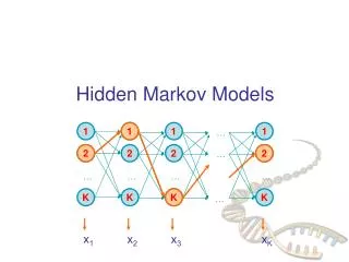
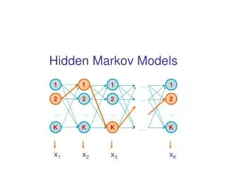
1 2 2 1 1 1 1 … 2 2 2 2 … K … … … … x1 K K K K x2 x3 xK … Hidden Markov Models
Substitutions of Amino Acids Mutation rates between amino acids have dramatic differences!
Substitution Matrices BLOSUM matrices: • Start from BLOCKS database (curated, gap-free alignments) • Cluster sequences according to > X% identity • Calculate Aab: # of aligned a-b in distinct clusters, correcting by 1/mn, where m, n are the two cluster sizes • Estimate P(a) = (b Aab)/(c≤d Acd); P(a, b) = Aab/(c≤d Acd)
Probabilistic interpretation of an alignment An alignment is a hypothesis that the two sequences are related by evolution Goal: Produce the most likely alignment Assert the likelihood that the sequences are indeed related
A Pair HMM for alignments Model M 1 – 2 This model generates two sequences simultaneously Match/Mismatch state M: P(x, y) reflects substitution frequencies between pairs of amino acids Insertion states I, J: P(x), P(y) reflect frequencies of each amino acid : set so that 1/2 is avg. length before next gap :set so that 1/(1 – ) is avg. length of a gap M P(xi, yj) 1 – 1 – I P(xi) J P(yj) optional
A Pair HMM for unaligned sequences Model R Two sequences are independently generated from one another P(x, y | R) = P(x1)…P(xm) P(y1)…P(yn) = i P(xi) j P(yj) 1 1 J P(yj) I P(xi)
To compare ALIGNMENT vs. RANDOM hypothesis 1 – 2 Every pair of letters contributes: M • (1 – 2) P(xi, yj) when matched • P(xi) P(yj) when gapped R • P(xi) P(yj) in random model Focus on comparison of P(xi, yj) vs. P(xi) P(yj) M P(xi, yj) 1 – 1 – I P(xi) J P(yj) 1 1 J P(yj) I P(xi)
To compare ALIGNMENT vs. RANDOM hypothesis 1 – 2 Every pair of letters contributes: M • (1 – 2) P(xi, yj) when matched • P(xi) P(yj) when gapped R • P(xi) P(yj) in random model Focus on comparison of P(xi, yj) vs. P(xi) P(yj) M P(xi, yj) 1 – 2 1 – 2 (1 – ) ----------- (1 – 2) I P(xi) J P(yj) Equivalent! 1 1 J P(yj) I P(xi)
To compare ALIGNMENT vs. RANDOM hypothesis 1 – 2 Every pair of letters contributes: M • (1 – 2) P(xi, yj) when matched • P(xi) P(yj) when gapped R • P(xi) P(yj) in random model Focus on comparison of P(xi, yj) vs. P(xi) P(yj) M P(xi, yj)/ P(xi) P(yj) 1 – 2 1 – 2 (1 – ) ----------- (1 – 2) I 1 J 1 Equivalent! 1 1 J P(yj) I P(xi)
To compare ALIGNMENT vs. RANDOM hypothesis Idea: We will divide alignment score by the random score, and take logarithms Let P(xi, yj) s(xi, yj) = log ––––––––– + log (1 – 2) P(xi) P(yj) (1 – ) P(xi) d = – log ––––––––––––– (1 – 2) P(xi) P(xi) e = – log –––––– P(xi) =Defn substitution score =Defn gap initiation penalty =Defn gap extension penalty
The meaning of alignment scores • The Viterbi algorithm for Pair HMMs corresponds exactly to global alignment DP with affine gaps VM(i, j) = max { VM(i – 1, j – 1), VI( i – 1, j – 1), Vj( i – 1, j – 1) } + s(xi, yj) VI(i, j) = max { VM(i – 1, j) – d, VI( i – 1, j) – e } VJ(i, j) = max { VM(i, j – 1) – d, VI( i, j – 1) – e } • s(.,.) (1 – 2) ~how often a pair of letters substitute one another • 1/mean length of next gap • (1 – ) / (1 – 2) 1/mean arrival time of next gap
The meaning of alignment scores Match/mismatch scores: P(xi, yj) s(a, b) log –––––––––– (ignore log(1 – 2) for the moment) P(xi) P(yj) Example: DNA regions between human and mouse genes have average conservation of 80% • What is the substitution score for a match? P(a, a) + P(c, c) + P(g, g) + P(t, t) = 0.8 P(x, x) = 0.2 P(a) = P(c) = P(g) = P(t) = 0.25 s(x, x) = log [ 0.2 / 0.252 ] = 1.163 • What is the substitution score for a mismatch? P(a, c) +…+P(t, g) = 0.2 P(x, yx) = 0.2/12 = 0.0167 s(x, y x) = log[ 0.0167 / 0.252 ] = -1.322 • What ratio matches/(matches + mism.) gives score 0? x(#match) – y(#mism) = 0 1.163 (#match) – 1.322 (#mism) = 0 #match = 1.137(#mism) matches = 53.2%
The meaning of alignment scores • The global alignment algorithm we learned, corresponds to: • Find the most likely alignment under the 3-state pHMM • The score of an alignment corresponds to: • Log-likehood ratio between • P(best alignment| alignment model), and • P(sequences were generated independently)
Substitution Matrices BLOSUM matrices: • Start from BLOCKS database (curated, gap-free alignments) • Cluster sequences according to > X% identity • Calculate Aab: # of aligned a-b in distinct clusters, correcting by 1/mn, where m, n are the two cluster sizes • Estimate P(a) = (b Aab)/(c≤d Acd); P(a, b) = Aab/(c≤d Acd)
BLOSUM matrices BLOSUM 50 BLOSUM 62 (The two are scaled differently)
Conditional Random Fields A brief description of a relatively new kind of graphical model
1 1 1 1 … 2 2 2 2 … … … … … K K K K … Let’s look at an HMM again 1 Why are HMMs convenient to use? • Because we can do dynamic programming with them! • “Best” state sequence for 1…i interacts with “best” sequence for i+1…N using K2 arrows Vl(i+1) = el(i+1) maxk Vk(i) akl = maxk( Vk(i) + [ e(l, i+1) + a(k, l) ] ) (where e(.,.) and a(.,.) are logs) • Total likelihood of all state sequences for 1…i+1 can be calculated from total likelihood for 1…i by only summing up K2 arrows 2 2 K x1 x2 x3 xN
1 1 1 1 … 2 2 2 2 … … … … … K K K K … Let’s look at an HMM again 1 • Some shortcomings of HMMs • Can’t model state duration • Solution: explicit duration models (Semi-Markov HMMs) • Unfortunately, state i cannot “look” at any letter other than xi! • Strong independence assumption: P(i | x1…xi-1, 1…i-1) = P(i | i-1) 2 2 K x1 x2 x3 xN
1 1 1 1 … 2 2 2 2 … … … … … K K K K … Let’s look at an HMM again 1 • Another way to put this, features used in objective function P(x, ): • akl, ek(b), where b • At position i: all K2akl features, and all K el(xi) features play a role • OK forget probabilistic interpretation for a moment • “Given that prev. state is k, current state is l, how much is current score?” • Vl(i) = Vk(i – 1) + (a(k, l) + e(l, i)) = Vk(i – 1) + g(k, l, xi) • Let’s generalize g!!! Vk(i – 1) + g(k, l, x, i) 2 2 K x1 x2 x3 xN
“Features” that depend on many pos. in x i-1 i • What do we put in g(k, l, x, i)? • The “higher” g(k, l, x, i), the more we like going from k to l at position i • Richer models using this additional power • Examples • Casino player looks at previous 100 pos’ns; if > 50 6s, he likes to go to Fair g(Loaded, Fair, x, i) += 1[xi-100, …, xi-1 has > 50 6s] wDON’T_GET_CAUGHT • Genes are close to CpG islands; for any state k, g(k, exon, x, i) += 1[xi-1000, …, xi+1000 has > 1/16 CpG] wCG_RICH_REGION x7 x8 x9 x10 x1 x2 x3 x4 x5 x6
“Features” that depend on many pos. in x x7 x8 x9 x10 x1 x2 x3 x4 x5 x6 Conditional Random Fields—Features • Define a set of features that you think are important • All features should be functions of current state, previous state, x, and position i • Example: • Old features: transition kl, emission b from state k • Plus new features: prev 100 letters have 50 6s • Number the features 1…n: f1(k, l, x, i), …, fn(k, l, x, i) • features are indicator true/false variables • Find appropriate weights w1,…, wn for when each feature is true • weights are the parameters of the model • Let’s assume for now each feature has a weight wj • Then, g(k, l, x, i) = j=1…nfj(k, l, x, i) wj
“Features” that depend on many pos. in x x7 x8 x9 x10 x1 x2 x3 x4 x5 x6 Define Vk(i): Optimal score of “parsing” x1…xi and ending in state k Then, assuming Vk(i) is optimal for every k at position i, it follows that Vl(i+1) = maxk [Vk(i) + g(k, l, x, i+1)] Why? Even though at pos’n i+1 we “look” at arbitrary positions in x, we are only “affected” by the choice of ending state k Therefore, Viterbi algorithm again finds optimal (highest scoring) parse for x1…xN
1 2 3 4 5 6 … x1 x2 x3 x4 x5 x6 1 2 3 4 5 6 … x1 x2 x3 x4 x5 x6 “Features” that depend on many pos. in x • Score of a parse depends on all of x at each position • Can still do Viterbi because state i only “looks” at prev. state i-1 and the constant sequence x HMM CRF
How many parameters are there, in general? • Arbitrarily many parameters! • For example, let fj(k, l, x, i) depend on xi-5, xi-4, …, xi+5 • Then, we would have up to K | |11 parameters! • Advantage: powerful, expressive model • Example: “if there are more than 50 6’s in the last 100 rolls, but in the surrounding 18 rolls there are at most 3 6’s, this is evidence we are in Fair state” • Interpretation: casino player is afraid to be caught, so switches to Fair when he sees too many 6’s • Example: “if there are any CG-rich regions in the vicinity (window of 2000 pos) then favor predicting lots of genes in this region” • Question: how do we train these parameters?
Conditional Training • Hidden Markov Model training: • Given training sequence x, “true” parse • Maximize P(x, ) • Disadvantage: • P(x, ) = P( | x)P(x) Quantity we care about so as to get a good parse Quantity we don’t care so much about because x is always given
Conditional Training P(x, ) = P( | x)P(x) P( | x) = P(x, ) / P(x) Recall F(j, x, ) = # times feature fj occurs in (x, ) = i=1…N fj(k, l, x, i) ; count fj in x, In HMMs, let’s denote by wj the weight of jth feature: wj = log(akl) or log(ek(b)) Then, HMM: P(x, ) =exp[j=1…n wj F(j, x, )] CRF: Score(x, ) =exp[j=1…n wj F(j, x, )]
Conditional Training In HMMs, P( | x) = P(x, ) / P(x) P(x, ) =exp[j=1…n wjF(j, x, )] P(x) = exp[j=1…n wjF(j, x, )]=: Z Then, in CRF we can do the same to normalize Score(x, ) into a prob. PCRF( | x) = exp[j=1…n wjF(j, x, )]/ Z QUESTION: Why is this a probability???
Conditional Training • We need to be given a set of sequences x and “true” parses • Calculate Z by a sum-of-paths algorithm similar to HMM • We can then easily calculate P( | x) • Calculate partial derivative of P( | x) w.r.t. each parameter wj (not covered—akin to forward/backward) • Update each parameter with gradient descent! • Continue until convergence to optimal set of weights P( | x) = exp[j=1…n wjF(j, x, )]/ Z is convex!!!
Conditional Random Fields—Summary • Ability to incorporate complicated non-local feature sets • Do away with some independence assumptions of HMMs • Parsing is still equally efficient • Conditional training • Train parameters that are best for parsing, not modeling • Need labeled examples—sequences x and “true” parses (Can train on unlabeled sequences, however it is unreasonable to train too many parameters this way) • Training is significantly slower—many iterations of forward/backward


