Antialiasing Miniaturized Textures
360 likes | 506 Views
CSS 552 – Prof. Sung Daniel R. Lewis June 3, 2013. Antialiasing Miniaturized Textures. Textured Geometry. Eye. Image Plane. Texels and Pixels (1). Textures are composed of discrete texels:. Pixels are projected onto texture:. Texels and Pixels (2). Image credit: Heckbert.

Antialiasing Miniaturized Textures
E N D
Presentation Transcript
CSS 552 – Prof. Sung Daniel R. Lewis June 3, 2013 Antialiasing Miniaturized Textures
Textured Geometry Eye Image Plane Texels and Pixels (1) Textures are composed of discrete texels: Pixels are projected onto texture:
Texels and Pixels (2) Image credit: Heckbert
Texture Magnification • Image resolution higher than texture resolution • Pixel grid “denser” than texel grid
Texture Minification • Image resolution lower than texture resolution • Texel grid “denser” than pixel grid Pixel Footprint Texel Grid
Point Sampling • Color comes from texel that happens to be at the intersection position • Poor representation of pixel area • Temporal aliasing e.g. “blinking” • At right: How would the pixel coloration change as the camera or geometry moved? • Improved by supersampling to a degree—becomes expensive as the texel:pixel ratio increases
Aliasing from point sampling Image credit: Angel
(1a) camera moves back (1b) (2) Prefiltered Texel Averaging • How many? • What shape? • Reminder: pixel coverage is view- and scene-dependent (1a, 1b) • Pixels cover various numbers of texels even within the same frame (2) • Cannot know a priori what to average • All methods prefilter the texture to generate approximations of all possible pixel footprints
point sampling detail mipmapping detail Mipmapping • Invented by Lance Williams, seminal paper published in 1983 • MIP an acronym for multum in parvo, meaning “many things in a small place” • Well-supported in hardware Image credit: Williams
Mipmapping: How It Works (1) • Start with 2n×2n texture • Create n downsampled texture maps, where each map Mi is 25% of the size of map Mi-1 • Average four pixels into one • How should pixels be “averaged”? Hold that thought... • Mipmaps require only 33.3% of the memory of the original texture Image credit: Wikipedia(a)
Mipmapping: How It Works (2) • Pixel color derived from (u, v, d) triple, where d is the level of detail Image credit: Akenine-Moller et al.
Finding d • (a) d ∝ || longest_pixel_edge || • lpe = || longest_pixel_edge || • d = 1 - ( lpe / texture_width ) • (b) • dx = sqrt((Δu / Δx)2 + (Δv / Δx)2) • dy = sqrt((Δu / Δy)2 + (Δv / Δy)2) • d ∝ max(dx, dy) • e.g.: • d = (1 / sqrt(2)) × max(dx, dy, sqrt(2)) • Challenge: in ray tracing, all we have is a point–not enough to reconstruct the red quadrilateral or find dx/dy
d Using d • Derive two maps from d • Sample both at (u, v) and interpolate between the samples • Common to add/subtract a level of detail bias from d to tweak results. Specified by user.
Filtering Algorithms • When downsampling, want to eliminate high frequency information that cannot be reproduced, before it causes aliasing • Low-pass filter (LPF) • Pixel averaging, a.k.a. box filtering, is a bad LPF • Ideal LPF is sinc • sin(πx)/(πx) • Infinitely wide • Approximate sinc by multiplying it by a windowing function and cutting it off Purple: Ideal filter Yellow: Box filter Green: Kaiser filter Blue: Point sampling Image credit: Blow(a)
Brightness and Gamma Correction (1) • Human eye is more sensitive to darker shades than brighter ones • Linear encoding of color wastes space on bright shades that are indistinguishable • Hence, images store color non-linearly, which is then scaled exponentially by γ to become linear • Clinear = (Cstore)γ • Typically, 1.8 ≤ γ ≤ 2.8
Brightness and Gamma Correction (2) • Filtering should not reduce brightness (ideally) • However: • A = tc1γ + tc2γ + tc3γ + tc4γ • B = ((tc1 + tc2 + tc3 + tc4) / 4)γ • A > B • Fixed by converting texel colors to linear space (decode), filter that, and then convert back (encode) Image credit: Blow(b)
Brightness and Gamma Correction (3) Detail view of mipmapped textures direct filtering linear filtering Image credit: Blow(b)
Achilles’ Heel of Mipmapping • Mipmapping weakness: all pixel projections that do not vaguely approximate squares • Below: color of pixel (red outline) comes from all shaded texels—mostly error!
Aliasing from mipmapping Image credit: Angel
dv dv du du du Ripmapping • Extension of mipmapping generating rectangular maps • Requires 300% more memory than original texture • Rarely used today Image credit: Wikipedia(b)
Summed Area Tables • Invented by Frank Crow, seminal paper published in 1984 • Based on rectangles like ripmapping, but with a dissimilar algorithm • Limited hardware support Top: Point sampling Middle: Mipmapping Bottom: Summed area tables Image credit: Akenine-Moller et al.
(i, j) (0,0) m n Generating the SAT • n×m SAT for n×m texture • Each slot (i, j) holds the sum of all texels in rectangle between origin (0, 0) and (i, j) • Requires more bits per channel (16–32) than original texture color (8) • Efficiently computed in a single pass: • I(i,j) = tc(i,j) + I(i−1,j) + I(i,j−1) − I(i−1,j−1)
(0,0) jt jb il ir Finding Rectangle Color • Rs = I(il,jb) − I(ir,jt) − I(il,jb) + I(il,jt) • Ra = Rs / ((ir − il)(jb − jt))
(0,0) jt jb il ir Finding Rectangle Color • Rs = I(il,jb) − I(ir,jt) − I(il,jb) + I(il,jt) • Ra = Rs / ((ir − il)(jb − jt))
(0,0) jt jb il ir Finding Rectangle Color • Rs = I(il,jb) − I(ir,jt) − I(il,jb) + I(il,jt) • Ra = Rs / ((ir − il)(jb − jt))
(0,0) jt jb il ir Finding Rectangle Color • Rs = I(il,jb) − I(ir,jt) − I(il,jb) + I(il,jt) • Ra = Rs / ((ir − il)(jb − jt))
(0,0) jt jb il ir Finding Rectangle Color • Rs = I(il,jb) − I(ir,jt) − I(il,jb) + I(il,jt) • Ra = Rs / ((ir − il)(jb − jt))
v (ub, vb) (ua, va) (uc, vc) (ud, vd) u v v1 v2 v0 v3 u Finding the Bounding Box • umin = min(ua, ub, uc, ud) • umax = max(ua, ub, uc, ud) • vmin = min(va, vb, vc, vd) • vmax = max(va, vb, vc, vd) • Rectangle: • Vertice[0] = (umin, vmin) • Vertice[1] = (umin, vmax) • Vertice[2] = (umax, vmax) • Vertice[3] = (umax, vmin)
Interpolating SAT Rectangles • Instead of rounding bounding box vertices to integers, allow the corners to fall between texel boundaries • Find color of all boxes at neighboring texels and interpolate between them based on distance
Achilles’ Heel ofRipmapping and SATs • Weakness of rectangle-based methods is pixel projections that cut diagonally across the texture • Below: color of pixel (red outline) comes from the texels in the shaded bounding box—mostly error!
Unconstrained Anisotropic Filtering • Built on top of mipmapping • Find (approximate) the major axis of the pixel footprint • Sample the mipmap (trilinear interpolation) at least twice along the axis, more if the footprint is long • Unlike normal mipmapping, use the length of the shorter side to compute the d value • Supported by PC graphics cards since early 2000s
Not Herein Considered... • Non-color textures: most of the antialiasing techniques can be extended for textures of other types (e.g., bump maps) • Curved surfaces • Literal edge cases
Implementation Plan (1) • Focus on implementing basic mipmapping • “Color” textures only • Time allowing, will implement more • Use RayTracer framework, with MP4 as the starting point • Risk: do not have enough information to compute the size or shape of the pixel footprint • Substantial modifications required
Implementation Plan (2) • Must have additional intersections (either world space or uv space) down within GetTexile() • Deep stack; might be easiest to stuff extra information into the IntersectionRecord • ComputeImage() • ComputeShading() • GetDiffuse() • AttributeLookup() • TextureLookup() • GetTexile() • Naïve implementation: ray trace four extra intersections at the pixel corners • Better: shifting “box” of four intersection records • No more expensive, except edges
Image Credits • Akenine-Moller, Tomas; Eric Haines; Naty Hoffman. Real-Time Rendering (3rd ed.). • Angel, Edward. Interactive Computer Graphics. • Found at http://vip.cs.utsa.edu/classes/cs5113s2007/lectures/materials/TextureInterpolationExample.html • Blow, Jonathan (a). “Mipmapping, Part 1.” Game Developer Magazine Dec. 2001. • Blow, Jonathan (b). “Mipmapping, Part 2.” Game Developer Magazine Jan. 2002. • Heckbert, Paul. “Fundamentals of Texture Mapping and Image Warping.” Thesis. University of California, Berkeley, 1989. • Wikipedia (a). <http://en.wikipedia.org/wiki/Mipmap> • Wikipedia (b). <http://en.wikipedia.org/wiki/Anisotropic_filtering> • Williams, Lance. “Pyramidal Parametrics.” Computer Graphics 13.3 (1983).