Download
1 / 40
400 likes | 574 Views
Need for an accurate Reno velocity model to understand amplification in the Reno Basin. Aasha Pancha. Reno Area Basin ANSS stations: installed1989 - 2003. Reno Area Basin Abbott and Louie (2000). 1. M=4.4 12/02/2000. 2. M=4.49 06/03/2004. 1. M=4.4 12/02/2000.

E N D
Need for an accurate Reno velocity model to understand amplification in the Reno Basin Aasha Pancha
1. M=4.4 12/02/2000 2. M=4.49 06/03/2004
1D synthetic Green's functions, computed in a layered elastic solid using the generalized reflection and transmission coefficients (Luco and Apsel, 1983; Zeng & Anderson, 1995). • E3D – fourth order, 3D staggered grid elastic finite difference code (Larsen & Schultz [5]; Larsen & Grieger [6]). • 0.2 to 0.6 Hz frequency band. • Compare these simulations with the observed data
Velocity Model = MA 0.25 km grid
RFNV RFMA SKYF
1. M=4.4 12/02/2000 2. M=4.49 06/03/2004
Insignificant correlation with basin depth Correlation is significant at the 68% confidence level.
Basin Depth vs Travel Time Residuals Correlation is significant at the 98% confidence level.
Travel time residuals vs Fourier spectral amplification Correlation is significant at the 90% confidence level.
Correlation with Vs30 and Vs100 Vs100 (98%) Vs30 (94%)
X X X X X X
Blue = soil to rock (SR) horizontal spectral ratios. • Red = soil to rock (SRv) spectral ratios of the vertical components of motion. • Black = horizontal to vertical spectral ratios (HVSR) for individual stations. • The black dashed = ratio the SR and SRv mean response spectra.
RF10/RFNZ E N Z
SF02 E N Z
RF11/RFMA E N Z
RF07/SKYF E N Z
Summary • Good agreement is observed between the amplitudes of the data, and that of the 3D simulation. • E3D matches the durations in the data and may anticipate some of the later arrivals. The 1D code does not. • 3D basin effects are important and a 3D model is required to model ground motion within the Reno area basin. • Need for refinement on the velocity and basin structural model.
ID Parameters • Mo = 5.17E+22 dyne-cm Calculated: • Area = 0.894 km • Rise time = 0.69 seconds • Slip = 6.3 cm E3D Parameters • Grid spacing = 0.25 km • 77 by 99 km down to depth of 40 km • Rise time 0.7 seconds Gaussian STF • to = 0.5 seconds • Depth 11 km • dt = 0.015, t=4800 72 seconds
1. M=4.4 12/02/2000 0.2 to 0.6 Hz
Reno Area Basin ANSS stations:1989-2003 Abbott and Louie (2000)
Correlation with Vs30 and Vs100 Vs100 (98%) Vs30 (94%)
NGA models Campbell and Bozorognia (thin dashed line); Choi and Youngs (thin line); Boore and Atkinson (dashed-dot line)