Download
1 / 18
180 likes | 327 Views
Because we know that data values . have mean i ,. the sample mean. is an estimate of i . Similarly, the. overall sample mean. Corresponding to our probability model we have a data model. The key difference is that the data model makes no statement about the distribution of the errors.

E N D
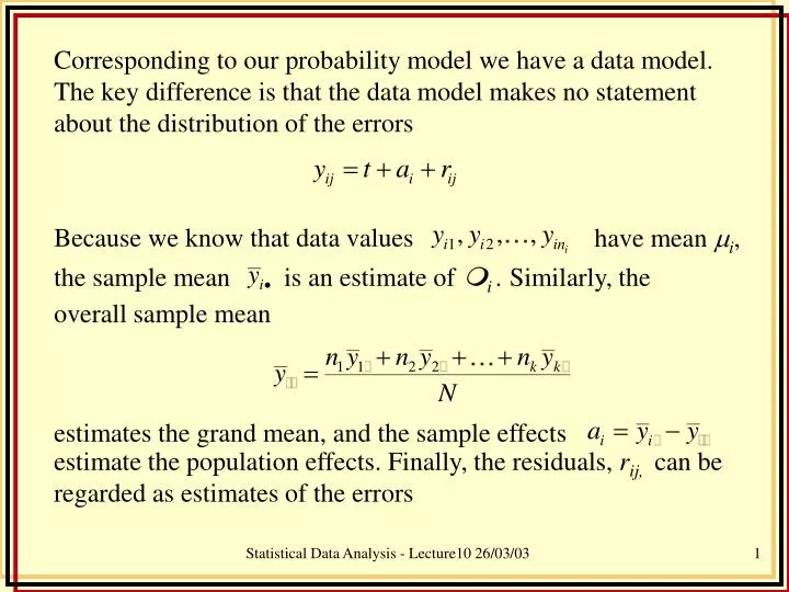
Because we know that data values have mean i, the sample mean is an estimate of i . Similarly, the overall sample mean Corresponding to our probability model we have a data model. The key difference is that the data model makes no statement about the distribution of the errors estimates the grand mean, and the sample effects estimate the population effects. Finally, the residuals, rij, can be regarded as estimates of the errors Statistical Data Analysis - Lecture10 26/03/03
With this notation, we can rewrite our model in a special way With a little rearrangement, we can write This says, if we ignore the grouping, the overall variability is measured by the size of the differences between the data and the grand mean, i.e. by the sum of the effects Statistical Data Analysis - Lecture10 26/03/03
With a little more manipulation, which we won’t reproduce, we can show that • We should be able to see that the left hand side (LHS) of the equation looks a lot like a standard deviation (the sum of the squared differences between the observation and the mean). • In fact is called the total sum of squares (TSS) and is a measure of overall variability in the data • On the right hand side (RHS) we have two terms. The first measures the variation due to intergroup differences, and is usally called the between group sum of squares (BGSS) • The second term measures variability between the observerations and the group means and is called the within group sum of squares (WGSS) Statistical Data Analysis - Lecture10 26/03/03
Using these new definitions we can rewrite our decomposition as Total sum of squares = Between group SS + Within group SS TSS = BGSS + WGSS • This is known as the Analysis of Variance Identity. • The ANOVA identity is helpful in thinking about our problem. • We wish to know if there is a diffference between the means • This is a relatively easy thing to do if we have a strong “signal” and low or weak “noise”, but not so easy to do if we have a weak signal or a proportionally large amount of noise • The BGSS tells us about the strength of the signal • The WGSS tells us about the level of the noise Statistical Data Analysis - Lecture10 26/03/03
In fact it can be shown that and Given we assumed normality of the errors, the (scaled) sums of squares have a chi-square distribution, and so the ratio of the sums of squares has an F distribution This leads us to the ANOVA table Statistical Data Analysis - Lecture10 26/03/03
One-way ANOVA table • The BGSS measures the total between group variability • WGSS measures the total within group variability. • We wish to have the average of both of these measures so we divide them by their respect degrees of freedom to get: • the between groups mean square (BGMS) and • the within groups mean square (WGMS). These are defined to be and Statistical Data Analysis - Lecture10 26/03/03
The P-value for the test is • We should recognise by now that the BGMS and the WGMS are chi-square random variables, hence a ratio of the two will have an F distribution. • Therefore our F-test statistic f0 is defined as the ratio of the BGMS to the WGMS, i.e. The sampling distribution of f0 under the assumption that the null hypothesis is true has been worked out and is called the F-distribution with k-1 numerator degrees of freedom and N – k denominator degrees of freedom. We write this as Statistical Data Analysis - Lecture10 26/03/03
The ANOVA table Nearly all computer packages that do statistics produce their ANOVA tables in a standard form. Statistical Data Analysis - Lecture10 26/03/03
A practical approach to one-way ANOVA • We’ve seen some of the theory, what do we do in practice? • Remember, ANOVA falls under the general hypothesis testing frame work. • Let’s work through the steps using the book data Statistical Data Analysis - Lecture10 26/03/03
Check model assumptions • Normally before we invest any effort in performing a hypothesis test, it pays to check some model assumptions. • If the model assumptions are met this assures the validity of the test results • I.e. If we know the model assumptions are okay than we can have some confidence that any significant results we find are not spurious Statistical Data Analysis - Lecture10 26/03/03
Model Assumptions for ANOVA • We’ve seen these before in various ways, but explicitly • Independence: The samples/groups are independent • Normality: The responses within a group are normally distributed • Equality of variance: The groups have the same variance or standard deviation Statistical Data Analysis - Lecture10 26/03/03
Independence of the groups • This assumption is absolutely crucial. If it is violated then then the results are meaningless • Statistical testing of this assumption is virtually impossible • However, if we know that the subjects are physically unrelated, then this is a reasonable guarantee of independence Statistical Data Analysis - Lecture10 26/03/03
Normality of the data • The assumption of normality is less crucial. • A relaxed constraint might be that the data are symmetric and unimodal • However, most experiments have very few observations in each group (In our experiment we have 50 observations per group which is unusually large),so checking this assumption can be difficult. • Usually, if the experiment is balanced, i.e. if there are an equal number of observations per group (ni = n i), then normality is not a big issue • If you do detect serious departures from normality (such as very skewed data) then a transformation of the data may be appropriate Statistical Data Analysis - Lecture10 26/03/03
Equality of variance • Recall our probability model • If our assumption of equality of variance does not hold, then any inferential statements we make may be flawed • We will never know whether the assumption is exactly true • The procedure is robust to small departures from this assumption • In general if the sample std. deviation of any group is ½ the size of the others then we might begin to be concerned about departures from this assumption • Transformation often cures these sorts of problems as well Statistical Data Analysis - Lecture10 26/03/03
Checking model assumptions • Plot the data – a boxplot is often a good start, although a jittered “dotplot” is good as well Statistical Data Analysis - Lecture10 26/03/03
Equalising variances • Both plots show that the data are right skewed • This violates the assumption of normality • Furthermore the spread of the data is different between the groups inequality of variance • We need to transform. How? Statistical Data Analysis - Lecture10 26/03/03
If the variances are unequal, then we can make an assumption that says that the std. deviation of each group is related to the mean by a power relationship of the form then, if we take logs we get a linear relationship Therefore, if we plot the logged std. deviations vs. the logged means and the relationship is approximately linear, then this is evidence that the power relationship holds. Furthermore, (and this is not immediately obvious) if the power relationship holds we transform to a power, p = 1 – b, then the std. deviations will be approximately equal Statistical Data Analysis - Lecture10 26/03/03