Download
1 / 36
360 likes | 578 Views
A Ghost Story Gluons and ghosts in the IR and the UV Berlin, June 15, 2009 Ph.,Boucaud, F De soto, J.-P. Leroy, A. Le Yaouanc, J. Micheli, O. Pène, J. Rodriguez-Quintero, A.Lokhov and C. Roiesnel. Gluons and ghosts in the IR: Lattice/Dyson-Schwinger Two solutions for Dyson Schwinger

E N D
A Ghost StoryGluons and ghosts in the IR and the UVBerlin, June 15, 2009Ph.,Boucaud, F De soto, J.-P. Leroy, A. Le Yaouanc, J. Micheli, O. Pène, J. Rodriguez-Quintero, A.Lokhov and C. Roiesnel Gluons and ghosts in the IR: Lattice/Dyson-Schwinger Two solutions for Dyson Schwinger The UV and MS The A2 condensate Scaling Conclusions
Infra-Red • Infra-red dog
QCD in the IR • QCD is « free » in the UV and confining in the IR. Hence the interest in IR behaviour. There exist different models for confinement which usually imply some consequences about the IR behaviour of Green functions. • Zwanziger’s conjecture that confinement has to do with Gribov horizon has such implications.
Existing tools ? • There are two sets of very usefus analytic relations to learn about QCD in the IR: Ward-Slavnov-Taylor (WST) identities and the infinite tower of Dyson-Schwinger (DS) integral equations. Lattice QCD give also essential numerical indications. The best would be to have an analytic solution, however this is not possible: • WST relates Green-Functions, not enough constraints. • DS are too complicated, highly non linear, it is not known how many solutions exist, but there is presumably a large number. Common way out ? • Use truncated DS with some hypotheses about vertex functions and sometimes compare the result to LQCD
WE PREFER 1- Combine informations from LQCD and analytic methods: not only using LQCD as an a posteriori check, but use it as an input for DSE. We believe that this allows a better control on systematic uncertainties of all methods. 2- Use WST identities (usually overlooked). This however leads today to an unsolved problem. 3- 1 and 2arecomplemented with mild regularity assumptions about vertex functions 4- Take due care of the UV behaviour (known since QCD is asymptotically free) and use a well defined renormalisation procedure (no renormalisation at =0 because of possible IR singularities).
Notations (In latin languages ghost is « fantômes, fantasmas ») • G(p2) is the bare gluon dressing function, = p2G(2)(p2), G(2)(p2) being the gluon propagator,G like gluon; Z3(2)= G(2)[MOM renormalisation constant of the gluon propagator] (frequent notation (fn): D(p2)instead of G(2)(p2)), • F(p2) is the bare ghost dressing function, = p2F(2)(p2), F(2)(p2) being the ghost propagator,F like fantôme; Z3(2)= F(2)[MOM renormalisation constant of the ghost propagator] (fn: G(p2)instead of F(2)(p2)) • In the deep IR it is assumed G(p2) (p2)G (fn: p2 D(p2) (p2)D or (p2)gl; G=2) • In the deep IR it is assumed F(p2) (p2)F (fn: p2 G(p2) 1/(p2)G or (p2)gh ; F=-) ~
Non-perturbative definitions of the strong coupling constant • Compute a three-gluon or ghost-ghost-gluon Green function, in a well defined kinematics depending on a scale , and the gluon and ghost propagators. • From there compute the corresponding bare vertex function B • Then: gR (2)= g0G(2)3/2 ’BorgR (2)= g0F (2) G (2)1/2 B • Special and preferred case (Von Smekal) : one vanishing ghost momentum. Taylor: B=1 gT (2)= g0F (2) G (2)1/2 T (2) = g02/(4)F (2)2 G (2) ~
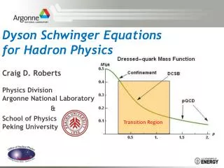
F(p2)2G(p2)is thus proportional to T (2) Lattice indicatesG ~1, F~ 0-, F(2)2G(2) 0, gf() 0 BUT A frequent analysis of the ghost propagator DS equation Leads to 2F + G=0(fn: D =2 G or gl=-2gl= 2) i.e. F(p2)2G(p2) ct and F(p2) In contradiction with lattice This is a strong, non truncated DS equation What is going on ?? Lattice gluodynamics computation of Landau gauge Green's functions in the deep infrared. I.L. Bogolubsky , E.M. Ilgenfritz, M. Muller-Preussker, A. Sternbeck arXiv:0901.0736
Two solutions to Ghost prop DSE • The non-truncated ghost propagator DS equation • It is also a WST equation !!! • We will first prove that there are two types of solutions, • 2F + G=0(fn: D =2G or or gl=-2gl= 2; « conformal solution ») F(p2)2G(p2) ct ≠0; In disagreement with lattice • F=0 (fn: G=0, « disconnected solution ») F(p2)ct ≠0In fair agreement with lattice, see recent large lattices: I.L. Bogolubsky, et al. arXiv:0710.1968 [hep-lat], A. Cucchieri and T Mendes arXiv:0710.0412 [hep-lat], and in agreement with WST • We will next show via a numerical study that solution I (II) are obtained when the coupling constant is equal (non-equal) to a critical value.
hep-ph/0507104, hep-ph/06040 • From anomalous dimensions it is easy to see that the loop is UV divergent. It needs a careful renormalisation (the subscript R stands for renormalised) or to use a subtracted DSE with two different external m omenta, thus cancelling the UV divergence. • 1/F-1/F’ = g2 ∫(G-G’)F ´ kinematics 2F + G=0 (I). But if F=F’ in the deep IR, i.e. if F ct ≠0, the dimensional argument fails since the power F does not appear in the lhs. This makes the point: 2F + G= 0 (I) unless F=0 • Solution (I) also imposes an additional constraint on the value of g2: • ~ • Z3 is the ghost prop renormalisation. It cancels the UV divergence. • When k 0 the lhs (k2)-F, Z3 is independent of k. • If F < 0, taking k0, Z3 has to be matched by the integral = g2 Integral(k=0), where g2=NcgR2z1 This leads to a well defined value for the coupling constant and the relation ~ ~
2F + G=0(fn: D =2 G), F(p2)2G(p2) ct ≠0,follows from a simple dimensional argument. • If F = 0, the same integral is equal to: -1/FR(0)=g2 Integral(k=0), the coupling constant now also depends on FR(0) which is finite non zero. In the small k region, FR(k2)=FR(0) + c (k2) ’F and now the dimensional argument gives ’F = G. If G=1then FR(k2)=FR(0) + c k2log(k2) To summarise, adding thatG(p2) 0(see lattice, late): • If F < 0, 2F + G=0, F(p2)2G(p2) ct ≠0and fixed coupling constant at a finite scale; G=-2F=2 From arXiv:0801.2762, Alkofer et al, -0.75 ≤F ≤-0.5, 1≤G≤1.5 II. if F = 0, F(p2)ct ≠0’F = G and no fixedcoupling constant Notice: solution II agrees rather well with lattice !!
Numerical solutions to Ghost prop DSE • To solve this equation one needs an input for the gluon propagator GR(we take it from LQCD, extended to the UV via perturbative QCD) and for the ghost-ghost-gluon vertex H1R: regularity is usually assumed from Taylor identity and confirmed by LQCD. • To be more specific,we takeH1R to be constant, and GR from lattice data interpolated with the G=1IR power. For simplicity we subtract at k’=0. We take =1.5 GeV.The equation becomes ~ ~ where F(k)=g () FR(k, ). Notice that F()=g(), with g defined as ~ ~ g2=NcgR2z1H1R= NcgB2Z3Z32H1B
~We find one and only one solution for any positive value of F(0). F(0)=∞ corresponds to a critical value: gc2 = 102/(FR2(0) GR(2)(0)) (fn: 102/(DR(0) lim p2GR(p2)) • This criticalsolution corresponds to FR(0)= ∞, It is the solution I, with2F + G=0, F(p2)2G(p2) ct ≠0, a diverging ghost dressing function and a fixed coupling constant. • The non-critical solutions, haveFR(0) finite, i.e. F = 0, the behaviour FR(k2)=FR(0) + c k2log(k2) has been checked. • Not much is changed if we assume a logarithmic divergence of the gluon propagator for k 0: FR(k2)=FR(0) - c’ k2log2(k2)
Ph. Boucaud, J-P. Leroy, A.Le Yaouanc, J. Micheli, O. Pene, J. Rodriguez--Quintero e-Print: arXiv:0801.2721 [hep-ph] gcrit2 = 33.198 • The input gluon propagator is fitted from LQCD. The DSE is solved numerically for several coupling constants. The resulting FR is compared to lattice results. For g2=29, i.e. solution II (FR(0)finite, F =0)the agreement is striking. The solution I (FR(0)infinite, 2F + G=0) , dotted line, does not fit at all. g2 = 29 g
F2(p)G(p): the dotted line corresponds to the critical coupling constant. It is solution I, goes to a finite non zero value at p 0; the full line corresponds to the g2 which fits best lattice data. It corresponds to Solution II, 2 F2(p)G(p) 0 when p 0.
Ghost and gluon propagator from lattice, (recent results) Gluon propagator Ghost dressing function Lattice gluodynamics computation of Landau gauge Green's functions in the deep infrared. I.L. Bogolubsky , E.M. Ilgenfritz, M. Muller-Preussker, A. Sternbeck arXiv:0901.0736 It resultsT (2) 2 when 0
Ghost and gluon propagator from lattice in strong coupling Ghost dressing function Strong coupling: =0
So what ? • Lattice favours solution II (finite ghost dressing function and vanishing coupling constant) • Possible loopholes in lattice calculations in the deep IR ? The discussion turns a little « ideological ». We should stay cautious about the deep infrared, but the trends are already clear around 300 MeV. Could there be a sudden change at some significantly smaller scale ? Why not ? But this looks rather far-fetched. • The Gribov-horizion based interpretation of confinement is then in bad shape. • Today we can’t say more
Ultra-Violet Theory stands here on a much stronger ground The issue is to compute QCD to be compared to Experiment. There are several ways of computing QCD. Is this under control ?
From T (2) to MS Compute T (2) = g02/(4)F (2)2 G (2) from there compute QCD __
__ MS (2/[GeV2]), quenched Only perturbation theory
__ MS (2/[GeV2]), quenched Adding a non perturbative c/p2 term to T (2) (A2 condensate) Only perturbation theory
<Aa Aa>condensate • <Aa Aa> is the only dimension-2 operator in Landau gauge. This makes it easier to apply Wilson expansion to different quantities. <Aa Aa> should be the same for all quantities and the Wilson coefficient is calculable. • T (2)= Tpert(2)(1+9/2 (Log(2/2))-9/44gT2/32 <A2>R • The Wilson coefficient has only been computed at leading log. • We vary the coefficient multiplying 1/2, compute MS(2) from Tpert(2)= Tlatt (2)/(1+c/2) using the three loop formula and fit c to get a plateau on the resulting MS(2) . • This gives both an estimate of MS and of<Aa Aa> Condensate Wilson coefficients
<Aa Aa>condensate • <Aa Aa> is the only dimension-2 operator in Landau gauge. This makes it easier to apply Wilson expansion to different quantities. <Aa Aa> should be the same for all quantities and the Wilson coefficient is calculable. • T (2)= Tpert(2) (1+9/2 (Log(2/2))-9/44gT2/32 <A2>R The Wilson coefficient has only been computed at leading log. • We vary the coefficient multiplying 1/2, compute MS(2) from Tpert(2)= Tlatt (2)/(1+c/2) using the three loop formula and fit c to get a plateau on the resulting MS(2) . • This gives both an estimate of MS and of<Aa Aa> Condensate Wilson coefficient
Lattice artefacts and scaling • Hypercubic artefacts: The dependence of any lattice quantity as a function of p2 is far from smooth, due to very different « geometries ». The H4 symmetry group of the lattice is only a subgroup of O(4). For example momenta 2(2,0,0,0)/L and 2(1,1,1,1)/L have the same p2 but are not related by H4 symmetry. • We define the H4 invariants p[2n]=p2n and expand, for example meas (p2,p[4],p[6],..) = T,latt (p2) + c4 a2p[4] + a4c6p[6] …. • This being done the dependence in p2 is very smooth below some limiting value of a2p2, but there are still O(4) invariant lattice artifacts Hyercubic improved Democratic Rawta
Lattice artifacts and scaling • In order to have enough lever arm to study the dependence in , we combine several lattice spacing. The finer lattice spacings allow to go higher momenta where 1/ 4 non-pertrubative contributions are reduced. • We match the plots using ratios of lattice spacing taken from r0, or we can fit the ratio of lattice spacings from the matching of T (2) from different lattice spacings. Both methods agree fairly well.
Different estimates of MS (2/[GeV2])quenched case • The non perturbative contribution is sizeable !!! T(2) ~ Tpert(2)(1+1.4/2) (1.4 % at 10 GeV) • There is a fair agreement from very different estimates.
Unquenched MS (2/[GeV2]) gT2<A2>=9.6(5) GeV2 Even larger than in quenched
Conclusions • IR: The ghost propagator Dyson-Schwinger equation allows for two types of solutions, • with a divergent ghost dressing functionand a finite non zero F2G, i.e. the relation 2F + G=0(fn: D =2 G), « conformal solution »; • with a finite ghost dressing functionand the relation F =0(fn: G =0), « decoupled solution » and a vanishing F2G Lattice QCD clearly favors II) • UV: T(2) is computed from gluon and ghost propagators. Discretisation errors seem under control. Perturbative scaling is achieved only at about 3 GeV (small lattice spacings) provided a sizeable contribution of <A2> condensate is taken into account. Different estimates of MSand of the condensate agree failry well. Extension under way to the unquenched case
Back-up slide What do we learn from big lattices ? Attilio Cucchieri, Tereza Mendes.Published in PoS (LATTICE 2007) 297. arXiv:0710.0412 [hep-lat] here G= - F (in our notations) = - gh I.L. Bogolubsky, E.M. Ilgenfritz, M. Muller-Preussker, A. Sternbeck Published in PoS(LATTICE-2007)290. arXiv:0710.1968 [hep-lat] They find F=-0.174 which seems at odds with both F=0 and F≤-0.5 But the fit is delicate, the power behaviour is dominant, if ever, only on a small domain of momenta.
Back-up slide comparison of the lattice data of ref arXiv:0710.1968 with our solution arXiv:0801.2721.
Back-up slideIR Ghost propagator from WST identitieshep-ph/0007088, hep-ph/0702092 • Assuming X regular when one momentum vanishes, the lhs is regular when r 0, then the ghost dressing has to be finite non zero: F(0) finite non zero, F=0 (fn: p2G(p2) finite≠0,G=0 or gh = 0, =0) • There is almost no way out, unless the ghost-gluon vertex is singularwhen only one momentum vanishes (difficult without violating Taylor’s theorem) • Does this contradict DS equations ? Lattice ? We do not believe, see later Cut lines: the external propagator has been cut; p,q,r : momenta Identities valid for all covariant gauges
Back-up slide IR Gluon propagator from WST identities, hep-ph/0507104, hep-ph/0702092 • : longitudinal propagator, the third gluon is transverse. Cut lines: the external propagator has been cut, p,q,r : momenta : gluons polarisation When q 0 it is easy to prove that the lhs vertex function vanishes under mild regularity assumptions. The rhs goes to a finite limit (see Taylor theorem).Then the transverse gluon propagator must diverge: G(2)(0)=∞, G<1(frequent notation: D(p2) ∞ D<1 or gl <1; < 0.5) or G=1with very mild divergences, to fit with lattice indications: G(2)(0) = finite≠0 unless The three gluon vertex diverges for one vanishing momentum. It might diverge only in the limit of Landau gauge. In arXiv:0801.2762, Alkofer et al, it is proven from DS that G >= 0, OK