Dynamic Programming
Dynamic Programming. Dynamic programming is a technique for solving problems with a recursive structure with the following characteristics:

Dynamic Programming
E N D
Presentation Transcript
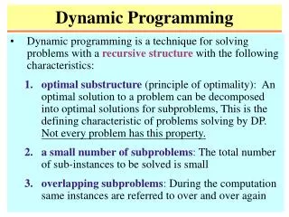
Dynamic Programming • Dynamic programming is a technique for solving problems with a recursive structurewith the following characteristics: • optimal substructure (principle of optimality): An optimal solution to a problem can be decomposed into optimal solutions for subproblems, This is the defining characteristic of problems solving by DP. Not every problem has this property. • a small number of subproblems: The total number of sub-instances to be solved is small • overlapping subproblems: During the computation same instances are referred to over and over again
y y x x ﹌﹌﹌ ﹌﹌﹌ ﹌﹌﹌ ﹌﹌﹌ u u v v y x Illustration If is the shortest path between u and v then is the shortest path between x and y
A Negative Example • Consider the problem of finding shortest paths on graphs that allow negative edge weights. Referring to the following graph, observe that a-b-c is a shortest path between a and c of length -2. However, unlike for the positive weight shortest path problem, the subpaths of this shortest path are not necessarily shortest paths. Thus, the shortest path between and and b is a-c-b (of length -1) not a-b (of length 1). The principle of optimality fails to hold for this problem. +2 +1 -3 a c b
The Airplane Problem • You live in a country with n+1 cities, all equally spaced along a line. The cities are numbered from 0 to n. You are in city n and want to get to 0. • You can only travel by plane. • You can only take one plane per day. The fare is determined by the distance (start city # - stop city #) you fly. Flying distance i costs air_fare[i]. • Spending the night in city i costs hotel_cost[i]. • Goal: Minimize the total cost to get to city 0. Ignore how many days it takes.
Example (n=4) i hotel_cost[i] air_fare[i] 1 2 1 2 2 4 3 5 9 4 0 16
A Divide and Conquer Solution function mincost(i: integer): integer; var k: integer; begin if i = 0 then return(0) else return( [air_fare[i-k]+hotel_cost[k]+mincost(k)]) end; /* mincost(n) is the answer */ • Let T(n)be the time required to solve a problem of size n. T(n) = T(i) + O(n), T(0) = O(1) T(n) - T(n-1) = T(n-1) + k, T(n) = 2T(n-1) + k for n > 1 T(n) = O(2n) !!! min 0 k i-1
A DP Solution A DP Solution var mincost: array[0..n] of integers begin mincost[0] := 0; for i := 1 to n do mincost[i]:= {(air_fare[i-k]+hotel_cost[k])+mincost[k]} end; /* the answer is in mincost[n] */ • This solution requires time Q(n2). min 0 k i-1
Observations • Original problem: Go from city n to city 0. • Generalized Problem: Go from city i to city 0. • Another generalized problem: Go from city n to city i. • Note: A more generalized problem is: "Go from city i to j (i ≥ j)". But this idea leads to a less efficient solution. • The method calculating one solution from some others is exactly the same as in the recursive version (except that function calls are replaced by array references). • Usually we get the idea for this method by thinking recursively. However, the final solution is iterative. • Divide and conquer: top-down. • Dynamic programming: bottom-up.
Matrix Multiplication • With the standard matrix multiplication method, how many scalar multiplications are needed for computing AB where A and B are of dimensions pq and qr? 1. pqr 2. pq2r
Chained Matrix Multiplication • Need to compute the product M = A1 A2 An of matrices A1, , An . By associativity (i.e., (AB)C = A(BC)) of multiplication we can compute M in various order. Use parentheses to describe the order. • The matrix-chain multiplication problem asks: What is the minimum cost for computing M?
Example • A is 10100, B 10010, and C 10100 (AB)C • How many operations for A(BC)? 200,000
Problem Formulation • A product of matrices is fully parenthesized if it is either a single matrix or the product of two fully parenthesized matrix products. • For example, for the product ABCD, there are five possible ways to fully parenthesize the product: (A(B(CD))), (A((BC)D)), ((A(BC))D), ((AB)(CD)), (((AB)C)D).
Problem Formulation • Now the matrix-chain multiplication problem is equivalent to: Given a list p = (p0,p1,,pn) of positive integers, compute the optimal-cost full-parenthesization of the chain (A1,A2,,An), where for each i, the ith matrix is of dimension pi-1 pi and the cost is measured by # of scalar multiplications.
Exhaustive Search • Is brute-force search efficient for this problem? • Let P(n) be the number of distinct full parenthesizations of n matrices. Then • Solving this, we obtain P(n) = C(n – 1), where • Thus, the brute-force search is too inefficient.
DP Approach: O(n3) • We need to cut the chain A1,, An somewhere in the middle, i.e., pick some k; 1 k n-1 and compute B(k) = A1,, Ak, C(k) = Ak+1,, An, and B(k)C(k). • Now, if we already know the optimal cost of computing B(k) and C(k) for all k; 1 k n-1, then we can compute the optimal cost for the entire product by finding a k that minimize “the optimal cost for computing B(k)" + “the optimal cost for computing C(k)" + p0pkpn • Use the same idea to compute the minimum costs for all the subproducts. This results in a bottom-up computation of optimal costs.
Generalization • Original problem: Compute the cost for A1A2An • Generalized problem: Compute the cost for AiAi+1Aj • For any k such that i ≤ k < j, divide product into two products: (AiAi+1Ak), (Ak+1Ak+2Aj). Let m[i, j] be the optimal cost for computing AiAi+1Aj. Then this grouping has cost m[i, k] + m[k+1, j] + pi-1pkpj • Then choose minimum for all such k. • For each i; j, 1 i j n, let s[i; j] be the smallest cut-point that provides the optimal cost for m[i, j].
Problem Ordering • To get a DP solution, order the problems: m[1,1] m[2,2] ... m[n-1,n-1] m[n,n] m[1,2] m[2,3] ... m[n-1,n] • • • m[1,n-1] m[2,n] m[1,n] • for i = 1 to n, set m[i; i] = 0. • for ℓ = 2 to n, compute s- and m-values for all length ℓ subchains (Ai,, Aj).
The Parenthesization • Once all the entries of s have been computed, we can compute the parenthesization that provides the optimal cost: • Print-Chain(i; j) • /* print the parenthesization for AiAj */ • print("(") • Print-Chain(i; s[i; j]) • Print-Chain(s[i; j] +1; j) • print(")")
Example • M1 M2 M3 M4 1020 2050 501 1100 m[1,1]=0 m[2,2]=0 m[3,3]=0 m[4,4]=0 m[1,2]=10000 m[2,3]=1000 m[3,4]=5000 m[1,3]=1200 m[2,4]=3000 m[1.4]=2200 • For example to compute m[1,4] choose the best of 20000 M1 (M2 M3 M4) 0 + 3000 + 20000 = 23000 0 3000 (M1 M2) (M3 M4) 10000 + 5000 + 50000 = 65000 10000 5000 (M1 M2 M3) M4 1200 + 0 + 1000 = 2200 1200 0 ((M1 (M2 M3)) M4)
Characteristics • optimal substructure: If s[1, n] = k, then an optimal full parenthesization contains those of (A1Ak) and (Ak+1An). • a small number of subproblems: The number of subproblems is the number of (i; j) with 1 i j n, which is n(n+1)/2 . • overlapping subproblems: m[i, j’] and m[i’, j] are referred to during the computation of m[i, j], for every i < i’ j and i j’ < j. • Because of the last property, computing an m-entry by recursive calls takes exponentially many steps.
Longest Common Subsequence • A sequence Z = <z1, z2, , zk> is a subsequence of a sequence X = <x1, x2, , xm> if Z can be generated by striking out some (or none) elements from X. • For example, <b, c, d, b> is a subsequence of <a, b, c, a, d, c, a, b> • The longest common subsequence problem is the problem of finding, for given two sequences X = <x1, x2, , xm> and Y = <y1, y2, , yn>, a maximum-length common subsequence of X and Y. • Brute-force search for LCS requires exponentially many steps because if m n, there are candidate subsequences
The Optimal-Substructure of LCS • For a sequence Z = <z1, z2, , zk> and i, 1 i k. let Zi denote the length i prefix of Z, i.e., Zi = <z1, z2, , zi>. • Theorem: Let X = <x1, , xm> and Y= <y1, , yn> • If xm = yn, then an LCS of Xm-1 and Yn-1 followed by xm (= yn) is an LCS of X and Y. • If xm yn, then an LCS of X and Y is either an LCS of Xm-1 and Y or an LCS of X and Yn-1.
Proof of the Theorem • Suppose xm and yn are the same symbol, say s. Take an LCS Z of X and Y. Generation of Z should need either xm or yn. Otherwise, appending s to Z would make a LCS. If necessary, modify the production of Z from X (from Y) so that its last element is xm (yn). Then Z is a common subsequence W of Xm-1 or Yn-1 followed by a s. By the maximality of Z, W should be an LCS. • If xm yn, then for any LCS Z of X and Y, generation of Z cannot use both xm and yn. So, Z is either an LCS of Xm-1 and Y or an LCS of X and Yn-1.
Computation Strategy • If xm = yn, then append xm to an LCS of Xm-1 and Yn-1. Otherwise, compute the longer of an LCS of X and Yn-1 and Xm-1 and Y. • Let c[i, j] be the length of an LCS of Xi and Yj. We get the recurrence: • Let b[i, j] maintain the choice made for (Xi, Yj). With the b-table we can reconstruct an LCS.
Example: • Here numeric entries are c-values and Arrows are b-values.
The Other 2 Characteristics of DP • a small number of subproblems: There are only (m+1)(n +1) entries in c (and in b). • overlapping subproblems: c[i; j] may be eventually referenced to in the process of computing c[i’, j’] for any i’ i and j’ j. • Time (and space) complexity of the algorithm : O(mn).
Optimal Polygon Triangulation • A polygonis a closed collection of lines (called sides) in the plane. A point joining two sides is a vertex. The line segment between two nonadjacent nodes is a chord. A polygon is convexif any chord is either on the boundary or in the interior of the polygon. • A polygon is represented by listing its vertices in counterclockwise order. • <v0, v1, , vn-1> represents the right polygon.
Triangulation • A triangulation of a polygon is a set T of chords of the polygon that divides the polygon into disjoint triangles. Every triangulation of an n-vertex polygon has n – 3 chords and divides the polygon into n – 2 triangles.
Optimal Triangulation • The weight of a triangle vivjvk, denoted by w(vivjvk), is |vivj| + |vjvk|+ |vkvi|, where |vivj| is the Euclidean distance between vi and vj. • The optimal (polygon) triangulation problem is the problem of finding a triangulation of a convex polygon that minimizes the sum of the weights of the triangles in the triangulation. • Given a triangulation with chords ℓ1, …, ℓn-3, the weight-sum can be rewritten as: • Note that vn = v0.
Observation • For each i, j, 0 i < j n, let Pij denote the polygon <vi, vi+1, , vj-1 , vj >, where either i > 0 or j < n. • The polygon Pij consists of j - i consecutive sides vivi+1, , vj-1vj and one more line vjvi which is a side if (i, j) = (0, n-1) or (1, n) and a chord otherwise. • Let t[i, j] be the sum of the chord length in an optimal triangulation of Pij. • The ultimate goal is to compute t[0, n-1].
The DP Approach • Idea: In any triangulation, there is a unique triangle that has vivj as a side. So, try each k, i < k < j, and cut the polygon by lines vivk and vjvk (one of these lines can be a side, but not both) thereby generating a triangle and the rest, which consists of one or two polygons.
The Key Step • Then the sum of the chord lengths are: • k = i +1: t[i +1, j] + |vi+1vj|. • k = j - 1: t[i, j -1] + |vivj-1|. • i +1 < k < j –1: t[i, k] + t[k, j] + |vivk| + |vjvk| • Pick a k that provides the smallest value.
The Algorithm • Let t(i, j) be the optimal cost of a triangulation of Pij. Observe: t(i; i) = 0 and for i < j, • Now a dynamic program algorithm is straightforward: just compute t(i, j)'s from small intervals (j – i) to large intervals for all i, j, and t(0, n-1) is the solution.
Optimal Binary Search Tree • Given a sorted list with n elements and the probability for accessing the keys (and leaves). Find the binary search tree with smallest cost. • Here, "leaves" are "fictitious" nodes, added to account for unsuccessful searches. • If p[i] is the prob. of node i, and q[i] is the prob. of an unsuccessful search between node i and i+1. The cost of a tree is: p[i]*level[node i]+ q[i]*(level[leaf i]-1)
The Idea • Let c(i, j) = minimum cost for tree consisting of nodes i, …, j. • In calculating c(i, j), we must find the best chance for the root. How to determine this? • Try all possibilities, k, i ≤ k ≤ j • Clearly, the 2 subtrees should be the optimal trees for the given set of nodes • Clearly, the cost of this tree is related to c(i, k-1) and c(k+1, j). However, the two subtrees have been "pushed down" one level.
Tree does not have to be balanced to be optimal • Analysis of the algorithm • Body of the loop takes time O(n) (finding minimun of ≤ n elements), and it is evaluated O(n2) times • Total O(n3)
CFG Parsing: CYK Algorithm • Problem: Given a context-free grammar G in Chomsky Normal Form, and a word w, decide if w is in L(G), the language generated by G. • Example: Given G, L(G) ={12n: n > 1}, by S AA, A BB | AA, B 1. • 16is in G by derivation: S AA AAA * BBBBBB * 111111. • Dynamic Programming solution: Exercise.

