Lecture 11 Stable Isotopes

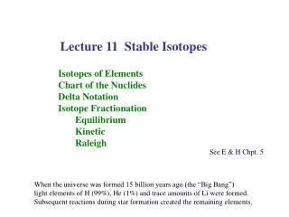
1. Lecture 11 Stable Isotopes Isotopes of Elements Chart of the Nuclides Delta Notation Isotope Fractionation Equilibrium Kinetic Raleigh See E & H Chpt. 5 When the universe was formed 15 billion years ago (the “Big Bang”) light elements of H (99%), He (1%) and trace amounts of Li were formed. Subsequent reactions during star formation created the remaining elements,

2. Isotopes of Elements The chemical characteristic of an element is determined by the number of protons in its nucleus. Atomic Number = # Protons = define the chemistry Different elements can have different numbers of neutrons and thus atomic weights (the sum of protons plus neutrons). Atomic Weight = protons + neutrons = referred to as isotopes There are 92 naturally occurring elements Some are stable; some are Radioactive

3. The chart of the nuclides (protons versus neutrons) for elements 1 (Hydrogen) through 12 (Magnesium). Valley of Stability Most elements have more than one stable isotope. b decay 1:1 line X X a decay Number of neutrons tends to be greater than the number of protons

4. Full Chart of the Nuclides 1:1 line

5. Examples for H, C, N and O: AtomicProtons Neutrons% Abundance Weight(Atomic Number) (approximate) Hydrogen H 1P 0N 99.99 D 1P 1N 0.01 Carbon 12C 6P 6N 98.89 13C 6P 7N 1.11 14C 6P 8N 10-10 Nitrogen 14N 7P 7N 99.6 15N 7P 8N 0.4 Oxygen 16O 8P 8N 99.76 17O 8P 9N 0.024 18O 8P 10N 0.20 1/2 = 5730 yr All Isotopes of a given element have the same chemical properties, yet there are small differences due to the fact that heavier isotopes typically form stronger bonds and diffuse slightly slower % Abundance is for the average Earth’s crust, ocean and atmosphere

6. Mass Spectrometer – Basic Schematics 1. Input as gases 2. Gases Ionized 3. Gases accelerated 4. Gases Bent by magnetic field 5. Gases detected Gases accelerated Gases ionized high vacuum Magnetic field deflects ion beam Detectors Isotopes are measured as ratios of two isotopes by various kinds of detectors. Standards are run frequently to correct for instrument stability

7. Nomenclature Report Stable Isotope Abundance as ratio to Most Abundant Isotope (e.g. 13C/12C) -Why? The Ratio of Isotopes is What is Measured Using a Mass Spectrometer The Ratio Can Be Measured Very Precisely. The isotope ratio of a sample is reported relative to a standard using d(“del”) notation – usually with units of ‰ because the differences are typically small. Define H = heavy L = light d (in ‰) = [(Rsample - Rstandard) / R standard ] x 1000 or R / Rstd = if δ is in ‰

8. Example: d13C (in %o) = [ (13C/12C)sample / (13C/12C) standard ] – 1 x 1000 Example: If (13C/12C) sample = 1.02 (13C/12C) std d13C = 1.02 (13C/12C) std / (13C/12C) std - 1 x 1000 = 0.02 x 1000 = 20 %o

9. Standards Vary

10. Isotopic Fractionation The state of unequal stable isotope composition within different materials linked by a reaction or process is called “isotope fractionation” Fractionation Factor = a aA-B = RA / RB where R = ratio of two isotopes in materials A or B often  = Rproducts / Rreactants

11. Two kinds of Isotope Fractionation Processes • Equilibrium Isotope effects • Equilibrium isotope fractionation is the partial separation of isotopes between two • or more substances in chemical equilibrium. • Usually applies to inorganic species. Usually not in organic compounds • Due to slightly different free energies for atoms of different atomic weight • Vibrational energy is the source of the fractionation. Equilibrium fractionation results from the reduction in vibrational energy when a more massive isotope is substituted for a less massive one. This leads to higher concentrations of the heavier isotope in substances where the vibrational energy is most sensitive to isotope fractionation (e.g., those with the highest bond force constants) • If molecules are able to spontaneous exchange isotopes they will exhibit slightly • different isotope abundances at thermodynamic equilibrium (their lowest energy state)

12. For example: exchange reactions between light = Al, Bl and heavy = Ah, Bh aA1 + bBh ↔ aAh + bB1 The heavier isotope winds up in the compound in which it is bound more strongly. Heavier isotopes form stronger bonds (e.g. think of like springs). If α = 1 the isotopes are distributed evenly between the phases. Example: equilibrium fractionation of oxygen isotopes in liquid water (l) relative to water vapor (g). H216O(l) + H218O(g) ↔ H218O(l) + H216O(g) At 20ºC, the equilibrium fractionation factor for this reaction is: α = (18O/16O)l / 18O/16O)g = 1.0098

13. Example: The carbonate buffer system involving gaseous CO2(g), aqueous CO2 (aq), aqueous bicarbonate HCO3- and carbonate CO32-. An important system that can exhibit equilibrium isotope effects for both carbon and oxygen isotopes 13CO2(g) + H12CO3-↔ 12CO2(g) + H13CO3- The heavier isotope (13C) is preferentially concentrated in the chemical compound with the strongest bonds. In this case 13C will be concentrated in HCO3- as opposed to CO2(g). For this reaction  has the form: H/L = (H/L)product / (H/L)reactants = (H13CO3- / H12CO3-) / (13CO2 / 12CO2) H/L = 1.0092 at 0ºC and 1.0068 at 30ºC

14. Example: Estimation of temperature in ancient ocean environments CaCO3(s) + H218O  CaC18OO2 + H2O The exchange of 18O between CaCO3 and H2O The distribution is Temperature dependent last interglacial Holocene last glacial d18O of planktonic and benthic foraminifera from piston core V28-238 (160ºE 1ºN) Planktonic and Benthic differ due to differences in water temperature where they grow. Assumptions: 1. Organism ppted CaCO3 in isotopic equilibrium with dissolved CO32- 2. The δ18O of the original water is known 3. The δ18O of the shell has remained unchanged Planktonic forams measure sea surface T Benthic forams measure benthic T

15. d18O in CaCO3 varies with Temperature from lab experiments E & H Fig 5.3

16. Complication: Changes in ice volume also influence d18O More ice, thus higher salinity – more d18O left in the ocean d18O increases with salinity

17. 2. Kinetic Fractionation Non-equilibrium – during irreversible reactions like photosynthesis Occurs when the rate of chemical reaction is sensitive to atomic mass Results from either differential rates of bond breaking or diffusion rates Compounds move at different rates due to unequal masses. Light are always faster. For kinetic fractionation, the breaking of the chemical bonds is the rate limiting step. Essentially all isotopic effects involved with formation / destruction of organic matter are kinetic There is always a preferential enrichment for the lighter isotope in the products. 12CO2 mw = 44 These must have the same kinetic energy (Ek = 1/2mv2) 13CO2 mw = 45 so 12CO2 travels 12% faster than 13CO2. All isotope effects involving organic matter are kinetic Example: 12CO2 + H2O = 12CH2O + O2 faster 13CO2 + H2O = 13CH2O + O2 slower Thus organic matter gets enriched in 12C during photosynthesis (d13C becomes negative)

18. Carbon Carbon has only two stable isotopes with the following natural abundances: 12C 98.89%o 13C 1.11%o Below are some typical d13C values on the PDB scale in %o. Standard (CaCO3; PDB) 0 Atmospheric CO2 -8 (was -6‰, getting lighter due to new CO2) Ocean SCO2 +2 (surface) 0 (deep) Plankton CaCO3 +0 (same as seawater) Plankton organic carbon -20 Trees -26 Atmospheric CH4 -47 Coal and Oil -26

19. δ13C in different reservoirs E & H Fig. 5.6

20. d13C of atmospheric CO2 versus time

21. Raleigh Fractionation - A combination of both equilibrium and kinetic isotope effects Kinetic when water molecules evaporate from sea surface Equilibrium effect when water molecules condense from vapor to liquid form Any isotope reaction carried out so that products are isolated immediately from the reactants will show a characteristic trend in isotopic composition. Example:Evaporation – Condensation Processes d18O in cloud vapor and condensate (rain) plotted versus the fraction of remaining vapor for a Raleigh process. The isotopic composition of the residual vapor is a function of the fractionation factor between vapor and water droplets. The drops are rich in 18O. The vapor is progressively depleted. Where Rvapor / R liquid = f (a-1) where f = fraction of residual vapor a = Rl/Rv Fractionation increases with decreasing temperature

22. Distillation of meteoric water – large kinetic fractionation occurs between ocean and vapor. Then rain forming in clouds is in equilibrium with vapor and is heavier that the vapor. Vapor becomes progressively lighter. dD and d18O get lower with distance from source. Water evaporation is a kinetic effect. Vapor is lighter than liquid. At 20ºC the difference is 9‰ (see Raleigh plot). The BP of H218O is higher than for H216O Air masses transported to higher latitudes where it is cooler. water lost due to rain raindrops are rich in 18O relative to cloud. Cloud gets lighter

23. d18O variation with time in Camp Century ice core. d18O was lower in Greenland snow during last ice age Effect of temperature Effect of ocean salinity 15,000 years ago d18O = -40‰ 10,000 to present d18O = -29‰ Reflects 1. d18O of precipitation 2. History of airmass – cumulative depletion of d18O

25. d13C in important geological materials

26. Influence of carbon source and kinetic fractionation on the average isotopic composition of marine and terrestrial plants.

27. Vertical profiles of SCO2, d13C in DIC, O2 and d18O in O2 North Atlantic data

29. d18O in average rain versus temperature

30. Meteoric Water Line linear correlation between dD and d18O in waters of meteoric origin

31. Spatial distribution of deuterium excess in the US