Download

1 / 44
460 likes | 999 Views
Statistical Tools for Multivariate Six Sigma. Dr. Neil W. Polhemus CTO & Director of Development StatPoint, Inc. Revised talk: www.statgraphics.comdocuments.htm. The Challenge. The quality of an item or service usually depends on more than one characteristic.

E N D
Statistical Tools for Multivariate Six Sigma • Dr. Neil W. Polhemus • CTO & Director of Development • StatPoint, Inc. • Revised talk: • www.statgraphics.com\documents.htm
The Challenge • The quality of an item or service usually depends on more than one characteristic. • When the characteristics are not independent, considering each characteristic separately can give a misleading estimate of overall performance.
The Solution • Proper analysis of data from such processes requires the use of multivariate statistical techniques.
Important Tools • Statistical Process Control • Multivariate capability analysis • Multivariate control charts • Statistical Model Building* • Data Mining - dimensionality reduction • DOE - multivariate optimization • * Regression and classification.
Example #1 • Textile fiber • Characteristic #1: tensile strength (115.0 ± 1.0) • Characteristic #2: diameter (1.05 ± 0.01)
Multivariate Capability Determines joint probability of being within the specification limits on all characteristics.
Mult. Capability Indices • Defined to give the • same DPM as in the • univariate case.
Hotelling’s T-Squared • Measures the distance of each point from the centroid of the data (or the assumed distribution).
Statistical Model Building • Defining relationships (regression and ANOVA) • Classifying items • Detecting unusual events • Optimizing processes • When the response variables are correlated, it is important to consider the responses together. • When the number of variables is large, the dimensionality of the problem often makes it difficult to determine the underlying relationships.
Reduced Models MPG City = 29.9911 - 0.0103886*Weight + 0.233751*Wheelbase (R2=73.0%) MPG City = 64.1402 - 0.054462*Horsepower - 1.56144*Passengers - 0.374767*Width (R2=64.3%)
Dimensionality Reduction • Construction of linear combinations of the variables can often provide important insights. • Principal components analysis (PCA) and principal components regression (PCR): constructs linear combinations of the predictor variables X that contain the greatest variance and then uses those to predict the responses. • Partial least squares (PLS): finds components that minimize the variance in both the X’s and the Y’s simultaneously.
Component Weights C1 = 0.377*Engine Size + 0.292*Horsepower + 0.239*Passengers + 0.370*Length + 0.375*Wheelbase + 0.389*Width + 0.360*U Turn Space + 0.396*Weight C2 = -0.205*Engine Size – 0.593*Horsepower + 0.731*Passengers + 0.043*Length + 0.260*Wheelbase – 0.042*Width – 0.026*U Turn Space – 0.030*Weight
PLS Coefficients • Selecting to extract 3 components:
Design of Experiments • When more than one characteristic is important, finding the optimal operating conditions usually requires a tradeoff of one characteristic for another. • One approach to finding a single solution is to use desirability functions.
Example #3 • Myers and Montgomery (2002) describe an experiment on a chemical process (20-run central composite design):
Desirability Functions • Maximization
Desirability Functions • Hit a target
Combined Desirability • di = desirability of i-th response given the settings of the m experimental factors X. • D ranges from 0 (least desirable) to 1 (most desirable).
Desirability Contours • Max D=0.959 at time=11.14, temperature=210.0, and catalyst = 2.20.
References • Johnson, R.A. and Wichern, D.W. (2002). Applied Multivariate Statistical Analysis. Upper Saddle River: Prentice Hall.Mason, R.L. and Young, J.C. (2002). • Mason and Young (2002). Multivariate Statistical Process Control with Industrial Applications. Philadelphia: SIAM. • Montgomery, D. C. (2005). Introduction to Statistical Quality Control, 5th edition. New York: John Wiley and Sons. • Myers, R. H. and Montgomery, D. C. (2002). Response Surface Methodology: Process and Product Optimization Using Designed Experiments, 2nd edition. New York: John Wiley and Sons. • Revised talk: www.statgraphics.com\documents.htm