CMC3_Tahoe, April 27, 2019
CMC3_Tahoe, April 27, 2019. Modular Knot Construction with Smooth and Discrete Optimization. Carlo H. Séquin EECS Computer Science Division University of California, Berkeley. Basel, Switzerland. M N G. Logarithmic Spiral. Jakob Bernoulli (1654‒1705). Leonhard Euler (1707‒1783).


CMC3_Tahoe, April 27, 2019
E N D
Presentation Transcript
CMC3_Tahoe, April 27, 2019 Modular Knot Construction with Smooth and Discrete Optimization Carlo H. Séquin EECS Computer Science Division University of California, Berkeley
Basel, Switzerland M N G
Logarithmic Spiral Jakob Bernoulli (1654‒1705)
Leonhard Euler (1707‒1783) Imaginary Numbers
Geometry in every assignment . . . CCD TV Camera (1973) Soda Hall (1992) RISC 1 MicroChip (1982) 3D-Yin-Yang (2000)
More Recent Designs and Models “Hilbert Cube” “Klein Bottle” “Evolving Trefoil” “Pax Mundi”
My Fascination with Knots Figure-8 knot TorusKnot (3,5) Chinese Button Knots Modular, building-block knot models Bronze sculptures cast by Steve Reinmuth, Eugene, OR
First “LEGO Knots” Parts 2 types of end-caps; 3 curved connectors
What can we do with those 5 Parts? Wild and crazy “snakes”, or part of a Hilbert curve …
“Rhombic Borsalinos” Original and with twisted legs
Twisted Connector Pieces Enlarged connector pieces with 45º twist:add flanges: two different pieces (azimuth!) 4 pairs make a nice twisted ring (360º)
LEGO Knot Sculptures Trefoil (knot 31) Figure-8 Knot (knot 41)
Single-Module Knots Suppose we are restraining ourselves to using just one single module! Can we build elegant and symmetrical knots? Some previous work and inspiration . . .
Richard Zawitz: Museum Tangle (1982) • A deformable unit with 18 quarter-circle segments
Knots Made from ONE Module • Problems: too many elements, lack of symmetry, self-intersections, bad loop closure. M. Zawidzki & K. Nishinari (2013):
Forming Closed Loops Is Difficult ! M. Zawidzki & K. Nishinari:
A First Try on a Figure-8 Knot -module 12-gon profile, 30 bending angle Composed of 4×10 -modules (S4 symmetry) Does not properly close! ( 6 DoF )
Polygonal Cross Section Why NOT using round tubes: If program specifies a torsion angle of 37.18 degrees, how would a user make sure to get the right angle ? With a discrete n-gonal profile, there are a finite number of discrete clicks for the torsion angle. 16 clicks is a good compromise between finding the right angle and still having reasonable design freedom.
The Chosen -Module Geometry 16-gon cross section (finer control of torsion angles) 30°bending angle in module (fewer overall modules) 2/3’’ pipe radius; 2’’ bending radius (“wiggle space”)
Tightest Closed Toroidal Ring Could just fit two more branches through the tunnel!
A First Batch of 20 Modules Out of the “Uprint” FDM machine from Stratasys
Modular UnKnots The UnKnot Undulating Loops Figure-8 Loop (Torus) (24, 20 modules) “Infinity”
Exploiting Symmetry Branch-ends can always be brought into coincidence, BUT . . . . Build the whole trefoil from three C2-symmetrical branches.
Simplest “ModKnot”: K 31 Trefoil Knot: K 31; D3 symmetry; uses 33 modules. Only 5 torsion angles need to be specified.
Trefoil Knot Sculpture 33 modules, D3 symmetry.
Modular Figure-8 Knot, K 41 Figure-8 Knot: K 41; S4 symmetry; uses 40 modules Even with the computer plan, this is difficult to assemble!
Figure-8 Knot Sculpture 40 modules, S4 symmetry
Cinquefoil Knot: K 51 D5 symmetry 50 modules
Designing More Complicated Knots What if one wants to build a more complicated knot, where there are a dozen or more unique torsion angles? Couldn’t a computer program do the work? Let’s tackle the simpler problem first: assume tubular module has circular cross sections. This seems harder: Infinitely many possible angles ! But it is actually simpler, because we have a smooth, continuous optimization space, where we can use gradient descent optimization.
Knot Design for Circular Cross Section Describe the knot to be realized with a smooth curve, e.g., defined by some spline curve. Sample that curve with as many points as you think you need to use number of modules.Each sample point then is the center of a module; neighboring modules join their ends exactly half-way between two sample points. Adjust the positions of all those points so that:neighbors are separated by exactly 2L (leg-length) andbending angles between subsequent segments are 30.
Computer Optimization Point distances must all be the 60 mm. Bending angles must all be 30 degrees. Move all the points around (in x,y,z)until all requirements are met everywhere. Symmetry: 15 Degrees of Freedom (DoF)
The Error (“Cost”, “Penalty”) Function • Try to minimize all the possible deviations listed in the previous slide: • Edge Length Differences (ELD): • ELD= ∑ (lengthi – 60mm)2 • Bending Angle Deviations (BAD): • BAD= ∑ (bending-anglei– 30)2 • Combine local errors into one overall error function: • COST= α * ELD + β * BAD { 0.5mm 1 }
The Error (or “Cost”) Surface Visible flaws= “Cost” Param. #1 Param. #2 Cost function is a “hilly landscape” over our 5-dimensional parameter space.(In the example above we only show 2 dimensions) In this “landscape” do gradient descent optimization (= follow a drop of water to the lowest point it can go to)
The Math behind Gradient Descent We could differentiate the total error function that I showed you earlier. Here it is not too bad; (sums of squared deviations from desired values). For any position of our rain drop, we can calculate the direction of the steepest descent in our cost landscape. Then we take a small step in that direction – and repeat the process.
Finding the Gradient by Sampling In mathematically more complex situations we may not have such a convenient closed-form expression to differentiate. Then we determine the gradient experimentally: Take a small step in “x” (axis of the first parameter)and see how much the cost function changes. ∆_cost / ∆_ step gives the slope in that direction. Do this for all parameters.
Gradient Descent in One Dimension error, cost, penalty ∆_ cost / ∆_ step = gradient. If our test step shows a cost increase, move in the opposite direction.
The Overall Gradient Overall, we would like to move in the direction that gives the largest cost reduction;i.e., move in the direction of the steepest gradient. So, we test the gradient in all DoFs: “x”, “y”, “z”, “w” … Form a vector that proportionally combines stepsin all possible directions byweighted them with the amount of cost reduction they provide.
Tricky Issues BAD! How large should the test step be to find the gradient reliably? Small enough to be in “linear range” Not so small that it is dominated by noise and rounding error.
Optimal Step Size? STEP TOO BIG! Once we have figured out the direction of the gradient, how big a step should we take in that direction? Again we would like to stay in the “linear” range:Half the step size should give roughly half the effect.
Using Gradient Descent • There may be no perfect solution . . .E.g. if trying to make a ring with only 11 segments: 3 30 30x30 = 900 deg.2 11x(3x3)= 99 deg.2 Error Minimization: By distributing it over all joints
Summary: Gradient Descent Not too difficult to implement! Normally works quite well. We can readily find solutions for circular tubing. But it would be difficult to actually use those results for a precise realization of a symmetrical knot. This is why we use an n-gonal cross section. But then gradient descent can no longer be used.
Adding Discrete Torsion Angles Allow only 16 legal torsion angles at any jointfor robustness of symmetrical knot configurations. Start as before with circular cross sections andreduce module separation and bending angle errors.These results will have arbitrary torsion angles;they could deviate from a “legal” value by 11.25. Thus we round all angles to their nearest legal valuesand set them as goals for a new optimization run. In this new optimization, we try to reduce the deviation from the legal torsion angles at a cost of increasing the deviations in module separation and bending angles.
Is this the best solution for our Knot? The rounding of the torsion angles was a rather dramatic change in knot geometry! Had we chosen slightly different “legal” values,would we have found a solution with lower overall error? To be sure, we should test neighboring combinations of legal torsion angles. BUT, this means making discrete changes:Gradient Descent does NOT work for this problem!
A Discrete Optimization Problem No smooth continuous moves; no gradient calculations possible. There are only discrete “moves”!One “click” in one torsion angle: cost function will take a jump! Any single such move will probably make matters worse; we may need a combination of several discrete moves to get an improvement. -- but what combinations?-- there is a very large set of possible combinations !
Discrete Optimization Techniques There are two techniques that you may want to know about: Simulated Annealing Genetic Algorithms Both are extensively used in industrial applications.
Genetic Algorithms Inspiration! 8 Variations from the central figure