Download
1 / 20
570 likes | 1.67k Views
Branch-and-Bound Traveling Salesperson Problem. The branch-and-bound problem solving method is very similar to backtracking in that a state space tree is used to solve a problem. The differences are that B&B does not limit us to any particular way of traversing the tree and

E N D
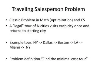
Branch-and-Bound Traveling Salesperson Problem
The branch-and-bound problem solving method is very similar to backtracking in that a state space tree is used to solve a problem. The differences are that B&B • does not limit us to any particular way of traversing the tree and • (2) is used only for optimization problems. A B&B algorithm computes a number (bound) at a node to determine whether the node is promising. The number is a bound on the value of the solution that could be obtained by expanding the state space tree beyond the current node.
Types of Traversal When implementing the branch-and-bound approach there is no restriction on the type of state-space tree traversal used. Backtracking, for example, is a simple type of B&B that uses depth-first search. A better approach is to check all the nodes reachable from the currently active node (breadth-first) and then to choose the most promising node (best-first) to expand next. An essential element of B&B is a greedy way to estimate the value of choosing one node over another. This is called the bound or bounding heuristic. It is an underestimate for a minimal search and an overestimate for a maximal search. When performing a breadth-first traversal, the bound is used only to prune the unpromising nodes from the state-space tree. In a best-first traversal the bound cab also used to order the promising nodes on the live-node list.
Traveling Salesperson B&B In the most general case the distances between each pair of cities is a positive value with dist(A,B) /= dist(B,A). In the matrix representation, the main diagonal values are omitted (i.e. dist(A,A) = 0).
Obtaining an Initial Tour Use the greedy method to find an initial candidate tour. We start with city A (arbitrary) and choose the closest city (in this case E). Moving to the newly chosen city, we always choose the closest city that has not yet been chosen until we return to A. Our candidate tour is A-E-C-G-F-D-B-H-A with a tour length of 28. We know that a minimal tour will be no greater than this. It is important to understand that the initial candidate tour is not necessarily a minimal tour nor is it unique. If we start with city E for example, we have, E-A-B-H-C-G-F-D-E with a length of 30
Defining a Bounding Heuristic Now we must define a bounding heuristic that provides an underestimate of the cost to complete a tour from any node using local information. In this example we choose to use the actual cost to reach a node plus the minimum cost from every remaining node as our bounding heuristic. h(x) = a(x) + g(x) a(x) - actual cost to node x g(x) - minimum cost to complete Since we know the minimum cost from each node to anywhere we know that the minimal tour cannot be less than 25.
Finding the Minimal Tour 1. Starting with node A determine the actual cost to each of the other nodes. 2. Now compute the minimum cost from every other node 25-4=21. 3. Add the actual cost to a node a(x) to the minimum cost from every other node to determine a lower bound for tours from A through B,C,. . ., H. 4. Since we already have a candidate tour of 28 we can prune all branches with a lower-bound that is ? 28. This leaves B, D and E as the only promising nodes. 5. We continue to expand the promising nodes in a best-first order (E1,B1,,D1).
5. We continue to expand the promising nodes in a best-first order (E1,B1,,D1).
6. We have fully expanded node E so it is removed from our live-node list and we have two new nodes to add to the list. When two nodes have the same bounding values we will choose the one that is closer to the solution. So the order of nodes in our live-node list is (C2,B1,B2,D1).
7. We remove node C2 and add node G3 to the live-node list. (G3,B1,B2,D1).
8. Expanding node G gives us two more promising nodes F4 and H4. Our live-node list is now (F4,B1,H4,B2,D1).
9. A 1st level node has moved to the front of the live-node list. (B1,D5,H4,B2,D1) 10. (H2,D5,H4,B2,D1) 11. (D5,H4,B2,D1) 12. (H4,B2,D1) 13. (B2,D1) 14. (H3,D1)
16.We have verified that a minimal tour has length >= 28. Since our candidate tour has a length of 28 we now know that it is a minimal tour, we can use it without further searching of the state-space tree.
Another Example In the previous example the initial candidate tour turns out to be a minimal tour. This is usually not the case. We will now look at problem for which the initial candidate tour is not a minimal tour. The initial tour is A-F-E-D-B-C-A with a total length of 32. The sum of the minimum costs of leaving every node is 29 so we know that a minimal tour cannot have length less than 29.
The live-node list is ordered by bounding value and then by level of completion. That is, if two nodes have the same bounding value we place the one that is closer to completion ahead of the other node. This is because the bounding value of the of the node closer to completion is more likely to be closer to the actual tour length.
The node shown in red were expanded from an active node (F3) with a possible tour length of 29. However the completed tours turned out to be significantly larger.
Expanding D3 we find an actual tour that is shorter than our initial tour. We do not yet know if this is a minimal tour but we can remove nodes from our live-node list that have a bounding value of >= 31. Now we expand D2 to find that it leads to tours of length >= 33.
Expansion of E2 eliminates this path as a candidate for a minimal tour.
When the live-node list is empty we are finished. In this example a minmal tour is A-C-E-D-B-F-A with a length of 31 we have found a tour that is shorter than the original candidate tour.