Download
1 / 30
300 likes | 425 Views
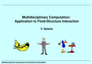
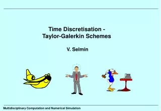
Unstructured Grids. Advancing Front Method. V. Selmin. Multidisciplinary Computation and Numerical Simulation. Advancing Front Method. • Elements, i.e. triangles and tetrahedra, and points are generated simultaneously. • Enables the generation of elements of variable size and stretching.

E N D
Unstructured Grids. Advancing Front Method. V. Selmin Multidisciplinary Computation and Numerical Simulation
Advancing Front Method • Elements, i.e. triangles and tetrahedra, and points are generated simultaneously. • Enables the generation of elements of variable size and stretching. • Differs from the approach followed in tetrahedral generators which are based upon Delaunay concepts which generally connect grid points which have already been distributed in space. • The generation problem consists of subdividing an arbitrarily complex domain into a consistent assembly of elements. • The consistency of the generated mesh is guaranteed if the generated elements cover the entire domain and the intersection between elements occurs only on common points, sides or triangular faces in the three dimensional case. • The process start by discretising each boundary curve. Nodes are placed on the boundary curve components and then contiguous nodes are joined with straight line segments. •In later stages of the generation process, these segments will become sides of some triangles. • The length of these segments must be consistent with the desired local distribution of mesh size. • This operation is repeated for each boundary curve in turn. Advancing Front Method
Advancing Front Method •Next stage consists of generating triangular planar faces. For each two dimensional region or surface to be discretised, all the edges produced when discretising its boundary curves are assembled into the so-called initial front. • The relative orientation of the curve components with respect to the surface must be taken into account in order to give the correct orientation to the sides in the initial front. The front is a dynamic data structure which changes continuously during the generation process. • At any given time, the front contains the set of all the sides which are currently available to form a triangular face. • A side is selected from the front and a tringular element is generated. This may involve creating a new node or simply connecting to an existing one. • After the triangle has been generated, the front is updated and the generation proceed until the front is empty. • The size and shape of the generated triangles must be consistent with the local desired size and shape of the final mesh. Advancing Front Method
Advancing Front Method • For the generation of tetrahedra, the advancing front procedure is taken one step further.. • The front is now made up of the triangular faces which are available to form a tetrahedron.. • The initial front is obtained by assembling the triangulations of the boundary surfaces. • Nodes and elements will be simultaneously created. • When forming a new tetrahedron, the three nodes belonging to a triangular face from the front are connected either to an existing node or to a new node. • After generation of a tetrahedron, the front is updated. • The generation procedure is completed when the number of triangles in the front is zero. Advancing Front Method
Curve Representation A support curve may be described by a piecewise parametric representation. In those representation, the curve is subdivided into arcs, and the position vector r of a generic point on each arc is expressed as a function of a single real parameter u, which by convention varies into the interval [0,1]. In general, this function is represented by a polynomial whose rank may change from arc to arc and which can be expressed as where each is a vector formed by three coefficients which represents the components of with respect to a cartesian reference system (x,y,z) , whereas n is the rank of the polynomial. The position vector can be rewritten as follows where and A point on the curve can then be identified by the number of the arc on which it is lying and the value of the parametric coordinates u, which is usually called local parametric coordinate. Advancing Front Method
Surface Representation The surfaces are represented by using a similar scheme. They are subdivided into patches which forms a regular grid on the so-called parametric plane. On this plane, we can define with respect fo each patch the local parametric coordinates u and v with varies on the interval [0,1]. The position r of a node on the surface can then be expressed as a polynomial expansion in u and v on each patch : The total rank of the polynomial is nxm, whereas n and m represent the rank of the polynomial with respect to the cartesian reference system (x,y,z): The position vector can be rewritten in the following form where The quantities U and V are expressed as Advancing Front Method
Characteristic Dimension Parameters The geometrical characteristics of an element can be defined in terms of the following mesh parameters. If n is the number of dimensions, the parameters used are a set of n orthogonal directions and n associated element sizes . The transformation T may be defined as the result of superposing n scaling operations with factor in each direction: Metric matrix→ Advancing Front Method
Characteristic Dimension Parameters The effect of the transformation T in two dimensions is illustrated for the case of constant mesh size throughout the domain. Advancing Front Method
Background Mesh Control over the mesh size characteristics is obtained by the specification of a spatial distribution of the mesh parameters by means of a background mesh. The background mesh is used for interpolation purposes only and is made up of triangles in two dimensions and tetrahedra in three dimensions Values of T are defined at the nodes of the background grid. At any point within an element of the background grid, the transformation T is computed by linearly interpolating its components from the element nodal values. The background mesh employed must cover the region to be discretised. In the generation of an initial mesh, the background mesh will usually consist of a small number of elements Advancing Front Method
Background Mesh The generation process is always carried out in the normalised space. The transformation matrix T is repeatedly used to transform regions in the physical space into regions in the normalised space In this way, the process is greatly simplified, as the desired size for a side, triangle or tetrahedra in this space is always unity. After the element has been generated, the coordinates of the newly created point, if any, are transformed back to the physical space using the inverse transformation. Interpolation within an element: Approximation by finite element: Select the element by using a search algorithm Compute the parametric coordinates by using the following linear/nonlinear equation, where are the coordinates of the node at which T has to be interpolated. Interpolate the matrix T at this point Advancing Front Method
Background Mesh Advancing Front Method
Curve Discretisation • The discretisation of the boundary curves is achieved by positioning nodes along the curves according to a • spacing dictated by a the local value of the mesh parameters. • Consecutive points are joined by straight lines to form sides. • In order to determine, the position and the number of nodes on each curve component, the following steps are • followed: • i- Subdivide each curve into smaller segments until their length is smaller that a certain prescribe value. • The length of each segment is computed numerically. • When subdividing a segment, the position and the tangent vectors corresponding to the new data points can • be found directly from the original definition of the segment. • ii- For all data points (i.e. those used to defined the curve and those created to satisfy the maximum • length criterion), interpolate from the background mesh the components of the transformation and • transform the position and the tangent vectors, i.e. • These new position and tangent vectors define a “curve” which can be interpreted as the image of the original • curve component in the normalised space. • Iii- Compute the length of the curve in the normalised space and subdivide it into segments of approximatively unit • lenght. • For each newly created points, identify the segment in which it is contained and its parametric coordinates. • This information is used to determine the coordinates of the new nodes in the physical space, by using • the curve component definition. Advancing Front Method
Triangle generation in two dimensional domain The triangle generation algorithm utilises the concept of a generation front. At the start of the process the front consists of the sequence of straight lines segments which connect consecutive boundary nodes. During the generation process, any straight line segment which is available to form an element side is termed active, whereas any segment that is no longer active is remove from the front. Thus, while the domain boundary will remain unchanged, the generation front changes continuously and needs to be updated whenever a new element is formed. Advancing Front Method
Triangle generation in two dimensional domain In the process of generating a new triangle the following steps are involved: i- Select a side AB of the front to be used as a base for the triangle to be generated. Here the criterion is to choose the shortest side. This is especially advantageous when generating irregular meshes. ii- Interpolate from the background grid the transformation T at the center of side denoted by M and apply these transformation to the nodes in the front which are relevant to the triangulation. The relevant points are defined to be all those that lies inside the circle of centre M and of a radius which is a multiple (3.0,…) of the side being considered. Let denote the positions in the normalised space of point A, B and M, respectively. iii- Determine, in the normalised space, the ideal position for the vertex of the triangular element. The point is on the line perpendicular to the side that passes through the point M and at a distance from the points A and B. The direction in which is generated is determined by the orientation of the side. Advancing Front Method
Triangle generation in two dimensional domain iii- The value of is chosen according to where L is the distance between points A and B. Only in situations where the side AB happens to have characteristics very different from those specified by the background mesh will the value of be different from unity. The above inequalities must be taken into account to ensure geometrical compatibility. iv- Select other possible candidates for the vertex and order them in a list. Two type of points are considered: a- all the nodes in the current generation front which are, in the normalised space, interior to a circle with centre and of radius , and b- the set of points generated along the height . Advancing Front Method
Triangle generation in two dimensional domain iv- A list is created which contains all the points with the furthest point from appearing at the head of the list. The points are added at the end of the list. v- Select the best connecting point. This is the first point in the ordered list which gives a consistent triangle. Consistency is guaranteed by ensuring that none of the newly created sides intersect with any of the existing sides in the front. vi- Finally, if a new node is created, its coordinates in the physical space are obtained by using the inverse transformation . vii- Store the new triangle and update the front by adding- removing the relevant sides. Advancing Front Method
Triangle generation in two dimensional domain Advancing Front Method
Triangle generation in two dimensional domain Mesh Quality Enhancement In order to enhance the quality of the generated mesh, two post- processing procedures may be applied. These procedures do not alter the total number of points or elements in the mesh. 1- Diagonal swapping: This changes the connectivities among nodes in the mesh without altering their position. This process requires a loop over all the element sides excluding those sides on the boundary. For each side AB common to the triangles ABC and ABD one considers the possibility of swapping AB by CD, thus replacing the two triangles ABC and ADB by the triangles ADC and BCD. The swapping is performed if a prescribed element quality criterion is satisfied better for the new configuration that by the existing one. 2- Mesh smoothing: This alters the positions of the interior nodes without changing the topology of the mesh. The element sides are considered as springs of stiffness proportional to the lenght of the side. The nodes are moved until the spring system is in equilibrium. The equilibrium positions are found by iterations. Each iteration amounts to performing a loop over the interior points and moving their coordinates to coincide with those of the centroid of the neighbouring points. Usually three iterations are performed. Advancing Front Method
v r(u,v) u Surface Discretisation The method followed for the triangulation of surfaces components is an extension of the mesh generation procedure for planar domains . The discretisation of each surface component is accomplished by generating a two dimensional mesh of triangles in the parametric plane (u,v) and then using the mapping r(u,v). This mapping establishes a one to one correspondence between the boundary surface component on a region on the parametric plane (u,v). Thus, a consistent triangular mesh in the parametric plane will be transformed, by the mapping r(u,v), into a valid triangulation of the surface component. The construction of the triangular mesh in the parametric plane (u,v) using the two-dimensional mesh generator, requires the determination of an appropriate spatial distribution of the two-dimensional mesh parameters. These consist of a set of two mutually orthogonal directions and two associated element sizes . Advancing Front Method
v r(u,v) u Surface Discretisation The two dimensional mesh parameters in the (u,v) plane may be evaluated from the distribution of the three dimensional mesh parameters and the mapping. Let consider a point P* in the parametric plane of coordinates (u*,v*), its image on the surface will be r(u*,v*). The transformation matrix (2x2) in the parametric space is built according to Then it is possible to extract from , the value of the mesh parameters that will be used to discretise the parametric space. By using the mapping, the coordinates of the nodes on the surface components may be computed according to r(u*,v*) Advancing Front Method
Generation of Tetrahedra The starting point for the discretisation of the three dimensional domain into tetrahedra is the formation of an initial generation front. The initial front is the set of oriented triangles which constitutes the discretised boundary of the domain and is formed by assembling the discretised boundary surface components. The algorithm for generating tetrahedra is analogous to that described for the generation of triangles. However, in the three-dimensional case, the range of possible options at each stage is much wider and the number of geometrical operations increases considerably. Thus, the ability of the method to produce mesh and the efficiency of its implementation relies heavily upon the type of strategy selected. Advancing Front Method
Generation of Tetrahedra The generation of a generic tetrahedral element involves the following steps: i- Select a triangular face ABC from the front to be a base fror the tetrahedron to be generated. In principle, any face could be chosen, but it has been found that to be advantageous in practice to consider the smallest faces first. For this purpose, the size of the face is defined in terms of the size of its shortest height. ii- Interpolate from the background grid the transformation T at the centroid of face denoted by M and apply these transformation to the nodes in the front which are relevant to the triangulation. The relevant points are defined to be all those that lies inside the sphere of centre M and of a radius which is a multiple (3.0,…) of the maximum dimension of the face being considered. Let denote the positions in the normalised space of point A, B, C and M, respectively. iii- Determine, in the normalised space, the ideal position for the vertex of the tetrahedral element. The point lies on the line which passes through the point M and which is perpendicular to the face. The direction in which is generated is determined by the orientation of the face. Advancing Front Method
Generation of Tetrahedra iii- The location of is computed so that the average length of the three newly created side which join point with points A, B and C is unity. For faces whose size in the parametric plane is very different from unity, this step may have to be modified to ensure geometrical compatibility. Let be the maximum of the distances between point and points A, B and C. iv- Select other possible candidates for the vertex and order them in a list. Two type of points are considered: a- all the nodes in the current generation front which are, in the normalised space, interior to a sphere with centre and of radius , and b- the set of points generated along the height . A list is created which contains all the points with the furthest point from appearing at the head of the list. The points are added at the end of the list. Advancing Front Method
Generation of Tetrahedra v- Select the best connecting point. This is the first point in the ordered list which gives a consistent tetrahedron. Consistency is guaranteed by ensuring that none of the newly created sides intersect with any of the existing faces in the front, and that none of the existing sides in the front intersect with any of the newly created faces. vi- Finally, if a new node is created, its coordinates in the physical space are obtained by using the inverse transformation . vii- Store the new tetrahedron and update the front by adding- removing the relevant faces.
Example: multi-component airfoil A two-dimensional discretisation of the domain around a four component airfoil in landing configuration is here shown. The background mesh employed for the generation, consisting of a few elements only, has been superposed on the generated mesh. The mesh in the vicinity of the airfoils is nearly of constant size and varies rapidly away from the airfoils. Advancing Front Method
Example: regional jet aircraft The spacing is provided by means of elementary solids. They are representative of very simple shapes: spheres, cylinders, troncated cones, … The spacing and stretching are given at the center or on an axis related to the elementary solid. These quantities varies with the distances between the considered points in the space and the center or the axis of the elementary solid. Advancing Front Method
Example: regional jet aircraft Advancing Front Method
Data Structures One of the major concerns in unstructured mesh generation is the use of an appropriate data structure. In structured mesh generation this problem does not play such an important role since the nature of the point set is such that it maps to an array in the computer memory. (i, j, k) This is not the case for unstructured meshes where executing operations, for example, finding local neighbouring points to a given point, can be computationally expensive if an appropriate data structure is not used. Furthermore, to achieve the efficiency required of mesh generators the use of fast algorithms is mandatory. Much can be learnt from developments in the field of computer science. In many case, algorithm for fast searching of data, geometrical construction, etc. , have already been investigated by computer scientists. In mesh generation, there is often the necessity of answering queries of the following kind: - Mesh topologies queries: For instance, give the list of mesh sides connected to a given node. - Mesh geometry queries: For instance, give all the smallest side contained in a set of side. - Range search queries: For instance, find all the mesh nodes laying inside a certain portion of physical space as a sphere in 3D For the latter, an inefficient organisation of the node coordinate data will cause the looping over all the mesh nodes n. This situation is usually referred to by saying that the algorithm is O(n). A better layout may reduce the number of operations for that query to O(log2n), which considerable savings when n is large. Advancing Front Method
Data Structures The final decision to use a certain data structure may depend on many factors, the most relevant are: 1- the type of operations we wish to perform on the data 2- the amount of computer memeory available. Moreover the best data organisation for a certain type of operations, for instance searching if an item is present in a table, is not necessarily the most efficient one for other operations such as deleting that item from the table. As a consequence, the final choice is often a compromise. Arrays: An array is the most fundamental data structure. An array is a fixed number of data items which are stored contiguously and which are accessible by an index. Linked lists: The major advantage over arrays are that they can expand and shrink in size, in particular, their maximum size need not to be known in advance. It is easy to insert or delete a new node and there is a flexibility to arrange items efficiently. Tree: A tree is a finite set whose elements are called nodes, such that 1- there is a special node calles root, which is normally indicated by Troot; 2- the others nodes may be partitioned in n disjoint set, [T1, …,Tn], each of which is itself a tree, called subtrees of the root The simplest tree is one node. In this case, the node is called leaf node. Advancing Front Method
Data Structures A tree takes is name by the way it is usually represented. Actually, the most used representation, is an upside-down tree with the root at the top. The tree root is linked to the root of its subtrees and the branching continues until a leaf node is reached. The number of subtrees of a node is called degree of the node. A leaf node has a degree 0. A tree whose nodes have at most degree N is termed N-ary tree. An important case is that of binary trees. In a binary tree each node is linked to at most two children, normally called the left and right child, respectively. Heaps: Often, there is the necessity to keep track of the record in a certain set which contains the maximum (or minimum) value of a particular field, that is termed key. For example, in a 2D mesh generation porocedure, it is needed to keep track of the front side with the minimum length, while the front is changing. An information structure which answers this type of query is called a priority queue, and a particular data organisation which could be used for a priority queue is the heap. A heap is formally defined as a binary tree with the following characteristics If k is the key associated with a heap node and and are the keys associated to non-empty left and right subtree root respectively, the following relation holds The key associated to each node is not smaller than the key of any node of its subtree. As a consequence, the node with the largest key (with respect to the chosen ordering relation) is always the root of the heap. Advancing Front Method