Download

1 / 43
430 likes | 609 Views
Unit 21 Magnetic measurements and tools to control the production. Soren Prestemon and Paolo Ferracin Lawrence Berkeley National Laboratory (LBNL) Ezio Todesco European Organization for Nuclear Research (CERN). QUESTIONS.

E N D
Unit 21Magnetic measurements and tools to control the production Soren Prestemon and Paolo Ferracin Lawrence Berkeley National Laboratory (LBNL) Ezio Todesco European Organization for Nuclear Research (CERN)
QUESTIONS • How to measure magnetic field and harmonics ? What precision can be reached ? • Is it possible to use measurements as X-rays to see what is inside the coil ? • This would allow to determine the quality of the assembly, find defects …
CONTENTS 1. Magnetic measurements • Rotating coils 2. How to set control limits on the production • Detection of field anomalies 3. From field anomalies to assembly faults • The inverse problem - methods • Examples 4. Electrical shorts: localization through field anomalies
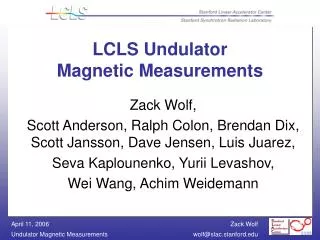
1. MAGNETIC MEASUREMENTS • Magnetic measurements devices • NMR/EPR principle • Hall probes • Flux measurements with pick-up coils • We only give an outline of the main methods • References • J. Billan “Performance of the Room Temperature Systems for Magnetic Field Measurements of the LHC Superconducting Magnets”, MT-19. • A. Jain, “Rotating coils”, Cern Accelerator School, Anacapri, CERN Yellow Report 1998-05. • L. Bottura, K. N. Henrichsen, “Field Measurements”, Cern Accelerator School, Erice, CERN Yellow Report 2004-008. • These slides are heavily relying on two lectures by A. Jain, USPAS 2006 in Phoenix: • Overview of magnetic measurement techniques • Harmonic coils
1. MAGNETIC MEASUREMENTS – NMR/EPR • Nuclear Magnetic Resonance (NMR) – Electron Paramagnetic Resonance (EPR) • The principle • A particle with spin and magnetic moment precesses in a magnetic field • The quantum energy levels are split, and the energy gap is proportional to the external magnetic field where is the gyromagnetic ratio • A radiofrequency energy is absorbed at frequencies corresponding to the energy gap • What is measured • The frequency at which one has the resonance absorption
1. MAGNETIC MEASUREMENTS – NMR/EPR • Nuclear Magnetic Resonance – Electron Paramagnetic Resonance • Different particles or atoms, having a different gyromagnetic ratio, are sensitive to different ranges of magnetic field • Example: electron has ~28 GHz/T, and is sensitive to 0.5 to 3.2 mT • Example: 2Hhas ~6.5 MHz/T, and is sensitive to 2 to 14 T • Absolute accuracy is high: 0.1 ppm (0.001 units) • Requirements • Field must be stable (<1% per second) • Field must be homogeneous (<0.1% per cm) • It is a standard for the absolute calibration of other systems
1. MAGNETIC MEASUREMENTSHALL PROBES • Hall probes • The principle • Charge carriers in a magnetic field experience a Lorentz force, which creates a voltage in the direction perpendicular to the field and to the current where G is a geometric factor, and RH is the Hall coefficient • What is measured • The voltage induced in the probe From A. Jain USPAS, Phoenix, 2006
1. MAGNETIC MEASUREMENTSHALL PROBES • Hall probes • Combination of Hall probes with a given geometry can deal with the issues of the angles between the probe and the field • Features • The range is large: 1 mT to 30 T • Accuracy is 0.01% to 1 % (1 to 100 units) • Dimensions are ~ mm • Frequency response is up to 20 kHz • Time stability is 10 units per year • Advantages: • Simple, cheap, commercially available, small, fast, suitable for complex geometries as detector magnets • Disadvantages: • Non-linear device, require elaborate calibration for each probe, sensitive to temperature, drift in long-term calibration
1. MAGNETIC MEASUREMENTSHALL PROBES • Flux measurements with pick-up coils • The principle • A variation of the magnetic flux through a coil induces a voltage • One can have either a time-dependent field with static coils, or moving coils (rotating coils) in a static magnetic field • What is measured • The voltage induced in the coil vs time • Integration over time and/or well controlled coil movement is needed From A. Jain USPAS, Phoenix, 2006
1. MAGNETIC MEASUREMENTSHALL PROBES • Flux measurements with pick-up coils • Features • Simple, passive, linear, drift-free device • Measurement of flux, not field knowledge of the coil surface and geometry is relevant, and limits the accuracy • Integration over the coil surface field variations along the surface are integrated harmonic analysis • Accuracy • Accuracy in main field can be ~ 50 ppm (0.5 units) • Accuracy in field direction can be ~ 0.05 mrad (0.5 units) • Field harmonics can be ~ 1 ppm (0.01 units) • Compensation (bucking) • An array with several loops of different geometries is used to improve the accuracy of measurements
1. MAGNETIC MEASUREMENTSHALL PROBES • Flux measurements with radial coils • Equations for the field in radial system • Radial coil is sensitive to tangential component • Making an FFT one can compute the multipoles • One can use a voltmeter, measuring the derivative of - in this case the speed must be uniform within 0.1% • One can use an integrator, measuring - one is independent of the rotational speed From A. Jain USPAS, Phoenix, 2006
1. MAGNETIC MEASUREMENTSHALL PROBES • Flux measurements with radial coils • The geometry of the rotating coils is more complicated • This is to improve the sensitivity • One uses more than one coil – some of them are summed to compensate automatically the main component and be more precise on the field harmonics LHC measuring coil for dipoles, courtesy of J. Billan HERA measuring coil for dipoles, from ???
CONTENTS 1. Magnetic measurements • Rotating coils • Stretched wire 2. How to set control limits on the production • Detection of field anomalies 3. From field anomalies to assembly faults • The inverse problem - methods • Examples 4. Electrical shorts: localization through field anomalies
2. HOW TO SET CONTROL LIMITS • Magnetic measurements carried out during the production phase have two distinct goals • Primary: check the obtained field quality versus the beam dynamics targets • Take corrective actions if some quantities exceed the target values (if possible) • Identify drifts • Secondary: evaluate the precision of the assembly through the uniformity of the magnetic field • A wrong component or assembly procedure will induce anomalies in the magnetic field • These anomalies in general can be tolerated by the beam (it is just one magnet, or part of it!) – but this could give performance limitations • Control limits should be independent of the beam dynamics targets • How to set them ?
2. HOW TO SET CONTROL LIMITS • How to set control limits for a large production • This is just a check of the uniformity of the final product – typical problem of all productions • Statistical approach • After having collected data of a few (~10) magnets, distributions of each field harmonics are analysed • Outliers due to known cases are removed • All the available information is used ! • High order multipoles, not relevant for the beam • Local multipoles – not only integral harmonics – not relevant for the beam (defect are usually local !) • Average and standard deviation are evaluated for each quantity • Control limits are set at - kis the number of sigma to be chosen • If the measurements fall outside, an anomaly is detected
2. HOW TO SET CONTROL LIMITS • Example: the LHC dipoles • Control sheet for the room temperature measurements of the collared coil • Limits set at 3-4 , and 6-8 • Quantities: • Main field • Field angle • Magnetic length • Multipoles up to 15 • Local harmonics !! (20 measured positions) • Separation straight part-heads • Separation average – variation along the length
2. HOW TO SET CONTROL LIMITS • The Lego model for FQ control • The right tower: high field at 1.9-4.4 K • Cold mass + cool-down (geometric) • Iron yoke saturation • Lorentz forces deformations • The left tower: injection at 1.9-4.4 K • Cold mass + cool-down (geometric) • Persistent currents • The second floor: cold mass at room temp. • Iron yoke effect • The first floor: collared coil at room temp. • Coil lay-out, assembly deformations • Each floor is controlled separately • Do not control cold mass, but (cold mass – collared coil), this is more precise Tokyo Town Hall, K.Tange associates
CONTENTS 1. Magnetic measurements • Rotating coils • Stretched wire 2. How to set control limits on the production • Detection of field anomalies 3. From field anomalies to assembly faults • The inverse problem - methods • Examples 4. Electrical shorts: localization through field anomalies
3. FROM FIELD ANOMALIES TO ASSEMBLY FAULTS • Once the field anomaly is detected, one has to understand the origin • First step: faulty measurement or defect in the magnet ? • Repetition of the measurements • Change of the measuring mole • Check of the consistency of data • Second step: heuristic methods • Longitudinal size of the anomaly correlated with length of components • The class of multipoles affected by the anomaly indicates the symmetry of the fault • If only allowed multipoles have anomalies, the defect has a up-down and top-bottom symmetry • If all classes of multipoles are affected, the defect should be only in one quadrant • Anomaly decay: defect close to the aperture affect all multipoles, defects far from the aperture affect only low orders (Biot-Savart)
3. FROM FIELD ANOMALIES TO ASSEMBLY FAULTS • Third step: try to solve the inverse problem • Method used for RHIC and LHC 1 - Build a library of the effect on multipoles of possible missing pieces (shims, …) or block movements compatible with mechanics 2 – Subtract from the field anomaly each effect, varying its amplitude 3 – If in one case the subtraction gives anomalies within three sigma (i.e. no anomaly), bingo ! • Remarks • The number of parameters (block movements) is large (~100) • The number of constraints is large (30 multipoles) • To avoid falling on unphysical solutions: • we do not try to bring the anomaly to zero, but within three sigma • we use only ‘possible’ movements • Drawback: we risk not to have imagined all possible defects • Other tool: use automatic codes to find solutions (e.g. Roxie, …)
3. FROM FIELD ANOMALIES TO ASSEMBLY FAULTS • Example – LHC main dipole 1027 • The field anomaly is large in absolute value – nearly 20 units !
3. FROM FIELD ANOMALIES TO ASSEMBLY FAULTS • We express the field anomaly as a ratio with respect to the sigma of the control limits – what we understand • Anomalies up to 11 sigma • In all multipoles classes (normal - skew, even - odd) the defect is asymmetric • Low orders only are affected – from order 5 on everything is normal
3. FROM FIELD ANOMALIES TO ASSEMBLY FAULTS • We plot the absolute values of the field anomaly in the semi-logarithmic scale • The slope of decay is not steep: defect looks at ~43 mm (inner radius of the outer layer coil)
3. FROM FIELD ANOMALIES TO ASSEMBLY FAULTS • We try our library of bad cases • Subtracting the effect of a missing shim (0.8 mm) on the outer layer, the anomaly disappears Field anomalies minus missing shim effect, expressed in units of sigma in the LHC main dipole 1027 Field anomalies/sigma in the LHC main dipole 1027
3. FROM FIELD ANOMALIES TO ASSEMBLY FAULTS • We convinced the firm to open the magnet • An outer layer shim was missing ! Picture from here, collars removed This is the shim This is the missing shim Missing shim in the LHC main dipole 1027
3. FROM FIELD ANOMALIES TO ASSEMBLY FAULTS • Example – LHC main dipole 2032 • The field anomaly is not so large in absolute value – 4 units at most
3. FROM FIELD ANOMALIES TO ASSEMBLY FAULTS • We express the field anomaly as a ratio with respect to the sigma of the control limits – what we understand • Anomalies up to 12 sigma • In all multipoles classes (normal - skew, even - odd) the defect is asymmetric • Low and high orders are affected
3. FROM FIELD ANOMALIES TO ASSEMBLY FAULTS • We plot the absolute values of the field anomaly in the semi-logarithmic scale • The slope of decay fits very well with a defect at ~28 mm (inner radius of the inner layer coil)
3. FROM FIELD ANOMALIES TO ASSEMBLY FAULTS • We tried our library of defects • Subtracting from the anomaly an inward movement of ~0.8 mm of block6 in one quadrant we go within three sigma in all multipoles (almost a miracle …) Field anomalies minus 0.75 mm block6 displacement expressed in units of sigma in the LHC main dipole 2032 Field anomalies expressed in units of sigma in the LHC main dipole 2032
3. FROM FIELD ANOMALIES TO ASSEMBLY FAULTS • We convinced the firm to open the magnet • It has been found that the coil was not glued and that block6 was detached from the inner layer • A more careful control of curing has been implemented Picture from here, collars removed Block6 inward displacement in the LHC main dipole 2032 Expected displacement in the LHC main dipole 2032
3. FROM FIELD ANOMALIES TO ASSEMBLY FAULTS • Example – LHC main dipole 1251 • The field anomaly is of the order of one unit on multipoles up to order 5 • Not so much indeed …
3. FROM FIELD ANOMALIES TO ASSEMBLY FAULTS • We express the field anomaly as a ratio with respect to the sigma of the control limits – what we understand • Very strong anomalies !! Up to 35 sigma • In all multipoles classes (normal - skew, even - odd) the defect is asymmetric • Higher orders are more affected
3. FROM FIELD ANOMALIES TO ASSEMBLY FAULTS • We plot the absolute values of the field anomaly in the semi-logarithmic scale • The slope of decay is not steep: defect looks at 28 mm (inner radius of the coil) or even inside … • Opened, the coil looked perfect … but the cold bore in the aperture had a magnetic permeability out of specification, producing the anomaly • A case impossible to simulate, heuristic methods provided a lot of info
3. FROM FIELD ANOMALIES TO ASSEMBLY FAULTS • We also had a few unexplained cases • The problem is difficult, remember … • Results for the LHC main dipole production (1276 magnets) • Errors identified with anomalies in warm magnetic measurements • 1 double coil protection sheet • 1 missing shim • 2 folded shims • 2 cold bores with anomalies in permeability • 1 wrong copper wedge • 8 cases of block6 movement due to bad coil curing • 15 magnets rescued at the level of collared coils (1.2% of the production) • RHIC has been the first case of application of magnetic measurements to control the production • Several cases found and rescued (wrong pieces …)
CONTENTS 1. Magnetic measurements • Rotating coils • Stretched wire 2. How to set control limits on the production • Detection of field anomalies 3. From field anomalies to assembly faults • The inverse problem - methods • Examples 4. Electrical shorts: localization through field anomalies
4. ELECTRICAL SHORTS: LOCALIZATION THROUGH MAGNETIC MEASUREMENTS • During the assembly procedures, the electrical resistance of the coil (copper) is measured in several steps • An inter-turn electrical short appears as a lower resistance of the coil • Voltage taps allow to detect the pole (upper or lower) but not the position • Electrical shorts create a field anomaly • This happens because the current is not flowing in some cables • This anomaly can be rather strong to be visible (i.e. larger than the control limits
4. ELECTRICAL SHORTS: LOCALIZATION THROUGH MAGNETIC MEASUREMENTS • Since in LHC main dipoles we have 20 measurements along the axis, we can find the longitudinal position of the short • Different classes of multiples are excited according to the layer (inner or outer) and to the position w.r.t. the connection side • A library of the effect of all possible inter-turn shorts can be created
4. ELECTRICAL SHORTS: LOCALIZATION THROUGH MAGNETIC MEASUREMENTS • Identification of the position in the cross-section • It is made by comparing the anomaly to the computed cases • Example: 2101 • Strong anomaly in a2b3 compatible with inter-turn short between conductors 34-34
4. ELECTRICAL SHORTS: LOCALIZATION THROUGH MAGNETIC MEASUREMENTS • Example: 2101 • Analysis of a4b5 confirm the result • The short is located in the first measuring position (head connection side) • Inspection allowed to find the short and cure it Measurement vs simulated shorts for the LHC main dipole 2101 Expected longitudinal position of the short for the LHC main dipole 2101
4. ELECTRICAL SHORTS: LOCALIZATION THROUGH MAGNETIC MEASUREMENTS • Results for the multilayer magnet production at BNL for HERA upgrade • First (?) case where the method has been applied • Identification of the short position has been successful • Repair has been possible [A. Jain, “Measurements as a tool to monitor production”, USPAS 2006] Repairing a magnet with an electrical short located through magnetic measurements, BNL
4. ELECTRICAL SHORTS: LOCALIZATION THROUGH MAGNETIC MEASUREMENTS • Results for the LHC main dipole production (1276 magnets) • 18 electrical shorts (1.5%) localized through warm magnetic measurements • Repair has been possible [B. Bellesia, et al., “Short circuit localization in the LHC main dipole coils by means of room temperature magnetic measurements', IEEE Trans. Appl. Supercond. (2006)]
CONCLUSIONS • We discussed how to measure field harmonics • Rotating coils, Hall probes, stretched wire • Precision can be very high (up to 1 ppm, 0.01 units) • We showed that room temperature magnetic measurements can be used as a tool to monitor production • Control limits: check of homogeneity of the production, not related to beam dynamics • Methods to read anomalies in magnetic measurements • Inverse problem – difficult ! • Use also heuristics methods • Build a library of all possible accidents you can imagine (and more …) • These methods have rescued several magnets in RHIC and LHC productions at a very early assembly stage • Big save of time and money ! • Electrical shorts can be localized with magnetic measurements
REFERENCES • Magnetic measurements • P. Schmuser, Appendix A and B • F. Asner, Ch. 13 • A. Jain et al, CERN 98-05 (1998) [a whole CAS dedicated to magnetic measurements] • L. Bottura, “Field measurements”, CERN 2004-008 (2004) 118-151. • Monitoring production, assembly faults • R.C. Gupta, et al., “Field Quality Analysis as a Tool to Monitor Magnet Production”, Proc. 15th International Conference on Magnet Technology (MT15), Science Press, Beijing, China (1997) 110. • C. Vollinger, E. Todesco, `Identification of assembly faults through the detection of magnetic field anomalies in the production of the LHC dipoles', presented at MT-19, IEEE Trans. Appl. Supercond. (2006). • B. Bellesia, et al., “Short circuit localization in the LHC main dipole coils by means of room temperature magnetic measurements', IEEE Trans. Appl. Supercond. (2006)


![Magnetic Measurements of MQW(B-A) [unit 10]](https://cdn1.slideserve.com/3252955/magnetic-measurements-of-mqw-b-a-unit-10-dt.jpg)