Download
1 / 36
360 likes | 377 Views
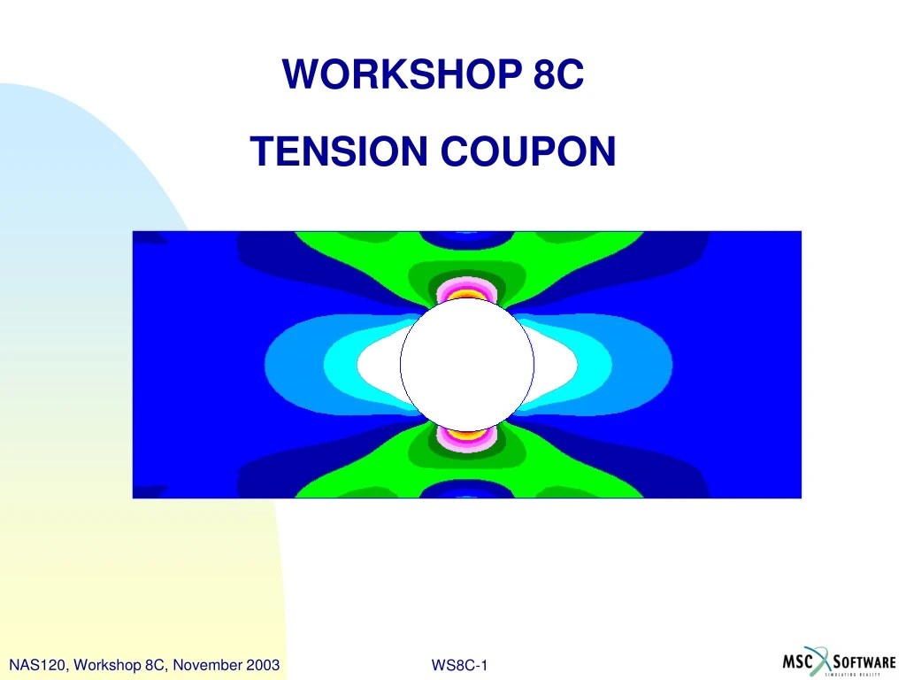
Learn how to analyze stress in a tension coupon using FEA. Build the geometry, control the mesh, and compare results to theoretical values.

E N D
WORKSHOP 8C TENSION COUPON NAS120, Workshop 8C, November 2003 WS8C-1
Problem Description • A tension coupon is constructed from aluminum with E = 10 x 106 psi and n = 0.3 • The coupon thickness is 0.125 in • An edge load of 50 lb is applied to the tension coupon
10 in 4 in 50 lb 2.0 DIA Hole
Workshop Objectives • Build the tension coupon geometry • Control the mesh by using techniques discussed in class • Compare FEA stress results to theoretical results From “Stress Concentration Factors” by R. E. Peterson, Figure 86: smax = 432 psi
Suggested Exercise Steps • Create a new database. • Create a geometry model of the tension coupon. • Use Mesh Seeds to define the mesh density. • Create a finite element mesh. • Verify the finite element mesh. • Define material properties. • Define element properties and apply them to the model. • Apply boundary conditions to the model. • Apply loads to the model. • Submit the model to MSC.Nastran for analysis. • Post Process results using MSC.Patran.
Step 1. Create New Database a a • Create a new database called tension_coupon.db • File / New. • Enter tension_coupon_c as the file name. • Click OK. • Choose Default Tolerance. • Select MSC.Nastran as the Analysis Code. • Select Structural as the Analysis Type. • Click OK. d e f b c g
Step 2. Create Geometry • Create two arcs • Geometry: Create / Curve / 2D ArcAngles. • Enter 0 for the Start Angle. • Enter 45 for the End Angle. • Enter [5 2 0] for the Center Point List. • Click Apply. • Repeat the procedure with 45 as the Start Angle and 90 as the End Angle. a b c d e
Step 2. Create Geometry Create two more curves. • Geometry: Create / Curve / XYZ. • Enter <0 2 0> for the Vector Coordinates List. • Enter [7 2 0] for the Origin Coordinates List. • Click Apply. • Repeat the procedure using <2 0 0> as the vector and [5 4 0] as the origin. a b c d
Step 2. Create Geometry f Create two surfaces • Geometry: Create / Surface / Curve. • Screen pick the top curve as shown. • Screen pick the upper arc. • Screen pick the right curve as shown. • Screen pick the lower arc. • Turn on display lines. b a d c e
Step 2. Create Geometry Create an extruded surface • Geometry: Create / Surface / Extrude. • Enter <3 0 0> as the Translation Vector. • Click in the Curve List box, then screen pick the right curve as shown. a c b
Step 2. Create Geometry Mirror the surfaces • Geometry: Transform / Surface / Mirror. • Set the Mirror Plane Normal to Coord 0.2. • For the Offset enter 2. • Click in the Surface List box. • Rectangular select all the surfaces as shown. a b c e d
Step 2. Create Geometry Mirror the surfaces again • Geometry: Transform / Surface / Mirror. • Set the Mirror Plane Normal to Coord 0.1. • For the Offset enter 5. • Click in the Surface List box. • Rectangular select all the surfaces as shown. a b c e d
Step 2. Create Geometry a The mirrored surfaces should look like the picture on the right. • Turn off display lines
Step 3. Create Mesh Seeds Create a uniform mesh seed • Elements: Create / Mesh Seed / Uniform. • Enter 3 for the Number of Elements. • Click in the Curve List box. • Screen pick each of the four edges on the left and right sides of the circle as shown. a d b c
Step 3. Create Mesh Seeds Create a biased mesh seed • Elements: Create / Mesh Seed / One Way Bias. • Enter 6 for the Number of Elements. • Enter 4 for L2/L1. • Click on the Curve List box. • Screen pick three of the remaining edges on the circle as shown. a e b c d
Step 3. Create Mesh Seeds Create a biased mesh seed • Elements: Create / Mesh Seed / One Way Bias. • Enter 6 for the Number of Elements. • Enter 0.25 (or -4) for L2/L1. • Click on the Curve List box. • Screen pick the 1 remaining edge on the circle. • Screen pick the horizontal edge to the right of the circle. a e f b c d
Step 3. Create Mesh Seeds The mesh seeds should agree with the picture on the right.
Step 4. Create Mesh Create a finite element mesh • Elements: Create / Mesh / Surface. • Set the Element Shape to Quad, Mesher to IsoMesh, and Topology to Quad4. • Click in the Surface List box. • Rectangular pick the surfaces as shown. • Enter 0.5 as the value for Global Edge Length. • Click Apply. a b d c e f
Step 4. Create Mesh Equivalence the model • Elements: Equivalence / All / Tolerance Cube. • Click Apply. a b
Step 5. Verify Mesh Verify the quality of the finite elements • Elements: Verify / Quad / All. • Click Apply. • Review the summary table. a c b
Step 5. Verify Mesh Perform specific quality tests on the elements. • Elements: Verify / Quad / Aspect. • Click Apply. • Review the fringe plot. • Repeat for Warp, Skew, and Taper tests. • Reset Graphics. a c d e b
Step 5. Create Material Properties Create an isotropic material • Materials: Create / Isotropic / Manual Input. • Enter aluminum as the Material Name. • Click Input Properties. • Enter 10e6 for the elastic modulus and 0.3 for the Poisson Ratio. • Click OK. • Click Apply. a d b c f e
Step 6. Create Element Properties Create element properties • Properties: Create / 2D / Shell. • Enter plate as the Property Set Name. • Click Input Properties. • Click on the Select Material Icon. • Select aluminum as the material. • Enter 0.125 for the thickness. • Click OK. a d f b c e g
Step 6. Create Element Properties Select application region • Click in the Select Members box. • Rectangular pick the surfaces as shown. • Click Add. • Click Apply. b a c d
Step 7. Apply Boundary Conditions Create the boundary condition • Loads/BCs: Create / Displacement / Nodal. • Enter fixed as the New Set Name. • Click Input Data. • Enter <0 0 0> for Translations and <0 0 0> for Rotations. • Click OK. a d b c e
Step 7. Apply Boundary Conditions Apply the boundary condition • Click Select Application Region. • Select the Curve or Edge filter. • Select the bottom left edge of the surface. • Click Add. • Select the top left edge of the surface. • Click Add. • Click OK. • Click Apply. b e f d c g a h
Step 7. Apply Boundary Conditions The boundary condition should agree with what’s shown on the right
Step 8. Apply Loads Create the load • Loads/BCs: Create / Total Load / Element Uniform. • Enter force as the New Set Name. • Set the Target Element Type to 2D. • Click Input Data. • Enter <50 0 0> for the Edge Load. • Click OK. a e b c d f
Step 8. Apply Loads Apply the load • Click Select Application Region. • For the application region select the right edge of the top right surface as shown. • Click Add. • Select the right edge of the bottom right surface. • Click Add. • Click OK. • Click Apply. b d c e a f g
Step 8. Apply Loads The loads and boundary condition should agree with what’s shown on the right.
Step 9. Run Linear Static Analysis Analyze the model • Analysis: Analyze / Entire Model / Full Run. • Click Solution Type. • Choose Linear Static. • Click OK. • Click Apply. a c b d e
Step 10. Post Process with MSC.Patran Attach the results file • Analysis: Access Results / Attach XDB / Result Entities. • Click Select Results File. • Choose the results file tension_coupon_c.xdb. • Click OK. • Click Apply. a c d b e
Step 10. Post Process with MSC.Patran a Erase geometry • Display: Plot/Erase. • Under Geometry click Erase. • Click OK. b c
Step 10. Post Process with MSC.Patran Create a Quick Plot of X Component Stress • Results: Create / Quick Plot. • Select Stress Tensor as the Fringe Result. • Select X Component as the Fringe Result Quantity. • Click Apply. • Record the maximum X component stress. Max X Stress = ________ a b c d
Step 10. Post Process with MSC.Patran a Turn off averaging • Results: Create / Fringe. • Select Stress Tensor as the Fringe Result. • Select X Component as the result quantity. • Click on the Plot Options Icon. • Change the Coordinate Transformation to CID. • Select Coordinate 0. • Change the Averaging Definition Domain to None. • Click Apply. d e f b g c h