Download
1 / 88
910 likes | 1.12k Views
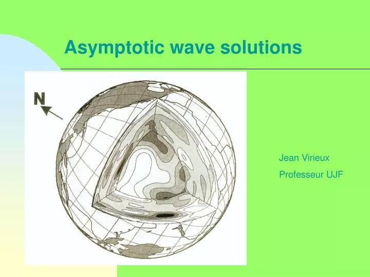
Asymptotic wave solutions. Jean Virieux Professeur UJF. Translucid Earth . S(t). Source. Same shape !. T(x). Travel-time T(x) Amplitude A(x). Receiver. Wavefront : T(x)=T 0. Wavefront preserved. Too diffracting medium : wavefront coherence lost !. Eikonal equation .

E N D
Asymptotic wave solutions Jean Virieux Professeur UJF
Translucid Earth S(t) Source Same shape ! T(x) Travel-time T(x) Amplitude A(x) Receiver Wavefront : T(x)=T0 Wavefront preserved Too diffracting medium : wavefront coherence lost !
Eikonal equation Two simple interpretation of wavefront evolution Orthogonal trajectories are rays T=cte Grad(T) orthogonal to wavefront Velocity c(x) DL T+DT Direction ? : abs or square
Transport Equation Tracing neighboring rays defines a ray tube : variation of amplitude depends on section variation
Ray evolution of x T=cte therefore evolution of We often note the slowness vector and the position Ray tracing equations s curvilinear abscisse Evolution of Evolution of is given by but Curvature equation known as the ray equation
System of ray equations with which ODE to select for numerical solving ? Either T or x sampling Many analytical solutions (gradient of velocity; gradient of slowness square)
Velocity variation v(z) Ray equations are The horizontal component of the slowness vector is constant: the trajectory is inside a plan which is called the plan of propagation. We may define the frame (xoz) as this plane. Where px is a constante For a ray towards the depth
Velocity variation v(z) At a given maximum depth zp, the slowness vector is horizontal following the equation zp If we consider a source at the free surface as well as the receiver, we get with p = usini In Cartesian frame In Spherical frame
Velocity structure in the Earth • Radial Structure
Main discontinuous boundaries • Crustal discontinuity (Mohorovicic (moho – 30 km) • Mantle discontinuity (Gutenberg – 2900 km) D’’ • Core discontinuity (Lehman – 5100 km) Shadow zone at the Gutenberg discontinuity: thickness of few kms
Minor discontinuities • Interface at 100-200 km • Interface at 670-700 km • Interface at 15 km (discontinuity of Conrad) These discontinuities are related to lithospheric, mesospheric and sismogenic structures. They are not expected to be deployed over the entire globe
System of ray equations Non-linear ODE ! with which ODE to select for numerical solving ? Either T or x sampling Many analytical solutions (gradient of velocity; gradient of slowness square)
Time integration of ray equations Runge-Kutta second-order integration Predictor-Corrector integration 1D sampling of 2D/3D medium : FAST stiffness receiver Initial conditions EASY source receiver Boundary conditions VERY DIFFICULT ? ? Shooting dp ? Bending dx ? Continuing dc ? source Save p conditions if possible ! AND FROM TIME TO TIME IT FAILS ! But we need 2 points ray tracing because we have a source and a receiver to be connected !
EikonalSolversFastmarchingmethod (FMM) (tracking interface/wavefront motion : curve and surface evolution) Layered medium Let us assume T is known at a level z=cte z=cte Compute along z=cte by a finite difference approximation z Deduce and extend T estimation at depth z+dz z + dz Assuming 1D plane wave propagation, we have been able to estimate T at a depth z+dz EIKONAL SOLVER From Sethian, 1999
Fast marching method (FMM) 2D case (tracking interface/wavefront motion : curve and surface evolution) Strategyavailable in 2D and 3D BUT only for the minimum time in eachnode in the spatial domain (x,y,z). Possible extension in the phase domain (for multiphases) ? Sharp interfaces are alwaysdifficult to handle in thisdiscrete formulation FromSethian, 1999 3D case Other techniques as fastsweepingmethods
Wavefronttracking Back-raytracingstrategy Once traveltime T iscomputed over the grid for one source, wemaybacktraceusing the gradient of T fromany point of the medium towards the source (shouldbeappliedfromeachreceiver) The surface {MIN TIME} isconvex as time increasesfrom the source : one solution ! A VERY GOOD TOOL FOR First Arrival Time Tomography (FATT) Smooth medium : simple case Ray Time over the grid
Ray tracing by wavefronts Rays and wavefronts in an homogeneous medium. (Lambaré et al., 1996)
Rays and wavefronts in a constant gradient of the velocity. (Lambaré et al., 1996)
Rays and wave fronts in a complex medium. (Lambaré et al., 1996)
Z in m 0 400 800 1200 1600 2000 (Lambaré et al., 1996)
Ray tracing by wavefronts Evolution over time : folding of the wavefront is allowed Dynamic sampling : undersampling of ray fans oversampling of ray fans Keep sampling of the medium by rays « uniform » Heavy task 2D & 3D ! Example of wavefront evolution in Marmousi model
Hamilton Formulation sympletic structure (FUN!) mechanics : ray tracing is a balistic problem Information around the ray Ray Meaning of the neighbooring zone – Fresnel zone for example but also anything you wish
Paraxial Ray theory does not depend on : LINEAR PROBLEM (SIMPLE) ! Estimation of ray tube : amplitude Estimation of taking-off angles : shooting strategy …
Practical issues Four elementary paraxial trajectories dy1t(0)=(1,0,0,0) dy2t(0)=(0,1,0,0) dy3t(0)=(0,0,1,0) dy4t(0)=(0,0,0,1) NOT A RAY !
Practical issues Paraxial rays require other conservative quantities : the perturbation of the Hamiltonian should be zero (or, in other words, the eikonal perturbation is zero) Point source conditions dqx(0)=dqz(0)=0 This is enough to verify this condition initially Solution From paraxial trajectories, one can combine them for paraxial rays as long as the perturbation of the Hamiltonian is zero. For a point source, a small slowness perturbation (a=10-4) gives a good approximate ray depending on the velocity variation in the medium: it is a kind of derivative ….
Practical issues Plane wave conditions dpx(0)=dpz(0)=0 This is enough to verify this condition initially Solution Two independent paraxial rays exist in 2D (while we have four elementary paraxial trajectories) Point paraxial ray Plane paraxial ray
Seismic attributes • 2 PT ray tracing non-linear problem solved, any attribute could be computed along this line : • Time (for tomography) • Amplitude (through paraxial ODE integration fast) • Polarisation, anisotropy and so on R A ray S Moreover, we may bend the ray for a more accurate ray tracing less dependent of the grid step (FMM) Log scale in time One ray Keep values of p at source and receiver ! Travel time evolution with the grid step : blue for FMM and black for recomputed time Grid step
Time error over the grid (0) Errors through rays deduced after FMM times Errors through FMM times NOT THE SAME COLOR SCALE (factor 100) Coarser grid for computation
ODE resolution • Runge-Kutta of second order • Write a computer program for an analytical law for the velocity: take a gradient with a component along x and a component along z Home work : redo the same thing with a Runge-Kutta of fourth order (look after its definition) Consider a gradient of the square of slowness
Runge-Kutt a integration Second-order integration Non-linear ray tracing Second-order euler integration for paraxial ray tracing
Four elementary paraxial trajectories dy1t(0)=(1,0,0,0) dy2t(0)=(0,1,0,0) dy3t(0)=(0,0,1,0) dy4t(0)=(0,0,0,1) Remember ! 3 is for point solution along x 4 is for point solution along z
Two points ray tracing: the paraxial shooting method Consider Dx the distance between ray point at the free surface and sensor position The estimation of the derivative is through paraxial computation We can compute an estimated Dq and, therefore, a new shooting angle
Amplitude estimation Consider DL the distance between the exit point of a ray and the paraxial ray running point. DL Thanks to the point paraxial ray estimation dq3 and dq4, we may estimate the geometrical spreading DL/Dq and, therefore, the amplitude A(r)
How to reconstruct the velocity structure ? • Forward problem (easy) from a known velocity structure, it is possible to compute travel times, emergent distance and amplitudes. • Inverse problem (difficult) from travel times (or similarly emergent distances), it is possible to deduce the velocity structure : this is the time tomography even more difficult is the diffraction tomography related to the waveform and/or the preserved/true amplitude.
Tomographic approach • Very general problem medicine; oceanography, climatology • Difficult problem when unknown a priori medium (travel time tomography) • Easier problem if a first medium could be constructed: perturbation techniques can be used for improving the reconstruction (delayed travel time tomography)
Travel Time tomography • We must « invert » the travel time or the emergent distance for getting z(u): we select the distance. • Abel problem (1826) Determination of the shape of a hill from travel times of a ball launched at the bottom of the hill with various initial velocity and coming back at the initial position.
x x dx ds y ABEL PROBLEM A point of mass ONE and initial velocity v0 reaches a maximal height x given by We shall take as the zero value for the potential energy: this gives us the following equations and its integration: We may transform it into the so-called Abel integral where t(x) is known and f(x) is the shape of the hill to be found: this is an integrale equation.
The exact inverse solution We multiply and we integrate We inverse the order of integration We change variable of integration We differentiate and write it down the final expression
THE ABEL SOLUTION By changing variable x in a-x and x in a-x, we get the standard formulae We must have t(x) should be continuous, t(0)=0 t(x) should have a finit derivative with a finite number of discontinuities. The most restrictive assumption is the continuity of the function t(x).
The solution HWB : HERGLOTZ-WIECHERT-BATEMAN From the direct solution, we can deduce the inverson solution After few manipulations, we can move from the Cartesian expression towards the Spherical expression We find r(v) as a value of r/v In Cartesian frame In Spherical frame
Stratified medium • We may find the interface at a depth h when considering all waves • We may reconstruct an infinity of structures with only direct and refracted waves. • We have a velocity jump when a velocity decrease
Velocity structure with depth • Velocity profile built without any a priori An difficulty arises when the velocity decreases.
An initial model through the HWB method • An initial model can be built • The exact inverse formulae does not allow to introduce additional information, F. Press in 1968 has preferred the exhaustive exploration of possible profiles (5 millions !). The quality of the profile is appreciated using a misfit function as the sum of the square of delayed times as well as total volumic mass and inertial moments well constrained from celestial mechanics ... • Exploration through grid search, Monte Carlo search, simulated annealing, genetic algorithm, tabou method, hant search …
A simple case : small perturbation • Initiale structure of velocity • Search of small variation of velocity or slowness • Linear approach