
Exploring Linear and Logistic Regression: Analyzing Insurance Claims Satisfaction
E N D
Presentation Transcript
Where Are We Going Today? • An Linear regressions example • Data how to obtain & manipulate it • Cleaning the data - Splus • Analysis • Issues • Interpretation • How to present the results meaningfully • Application • Description forecasting/prediction • Traps for the unwary • Logistic regression • Conclusions
An example? Insurance company claims satisfaction
Background: • Top secret company - insurance • Claims satisfaction • 546 persons asked to rate aspects of service and then overall satisfaction/likelihood to recommend – 5 point scale • We recommend 10 point scale - as more natural to respondents (1-10) • Major ‘storm in a teacup’
Questionnaire – explanatory variables • Thinking firstly about the service you received from (top secret). I am going to read you some statements about this service and as I read you each statement, please give your opinion using a five-point scale where 1 is extremely dissatisfied and 5 extremely satisfied • (read, rotate (start at x). write in (one digit) per statement) • How satisfied or dissatisfied are you with:. • ... everything being kept straightforward • ... being kept in touch while the claim was being processed • ... the general manner and attitude of the staff you dealt with • ... your claim being dealt with promptly • ... being treated fairly
Questionnaire – dependent variables 4a Using the same five-point scale as previously where 1 is extremely dissatisfied and 5 extremely satisfied, how satisfied or dissatisfied were you with the overall service you received from (Top secret) ? • write in (one digit) 4b And, using a five-point scale where 1 is extremely unlikely and 5 extremely likely, how likely or unlikely are you to recommend (Top secret) insurance to others? • write in (one digit)
Data • Get DP to create an Excel file with all the data • Make your self familiar with Excel formats • Clean data • Then start analysing the data • Use data to describe each aspect of service:… • the time taken to get an appointment with the loss adjustor • the convenience of meeting with the loss adjustor • the general manner and attitude of the loss adjustor you dealt with • being kept in touch while your claim was processed... • the time taken for repairs to be completed
### cleaning the data Regress.eg[,-1][Regress.eg[,-1]==6]_NA sum(is.na(Regress.eg)) [1] 49 mn_apply(Regress.eg,2,mean,na.rm=T) for (i in 2:ncol(Regress.eg)){ id_is.na(Regress.eg[,i]) Regress.eg[id,i]_mn[i] } ## let's look at this with a bit of jitter Regress.eg2_Regress.eg2+ matrix(rnorm(nrow(Regress.eg2)*ncol(Regress.eg2),0,.1),ncol=ncol(Regress.eg2)) Regress.eg2_Regress.eg2[,-1] ## perform a matrix plot on this puppy (use menus) Some Code for cleaning / inspecting
## let’s analyse this data apply(Regress.eg,2,mean) cor(Regress.eg2) Regress.eg.coeff_NULL for (i in 2:6){ Regress.eg.coeff_c(Regress.eg.coeff, lm(Regress.eg[,7]~Regress.eg[,i])$coeff[2]) } Regress.eg.mlr.coeff_lm(formula = Satisfaction ~ Straightforward + kept.in.touch + manner.attitude + prompt + fairly, data = Regress.eg, na.action = na.exclude)$coeff More Code
Output Code > Regress.eg.mlr.coeff (Intercept) Straightforward kept.in.touch -0.08951399 0.3802814 0.1624232 manner.attitude prompt fairly 0.08986848 0.2199223 0.1567801 > cbind(apply(Regress.eg, 2, mean)[2:6], cor(Regress.eg)[ 2:6, 7], Regress.eg.coeff, Regress.eg.mlr.coeff[ -1]) Regress.eg.coeff Straightforward 4.329650 0.7982008 0.8010022 kept.in.touch 4.394834 0.7280380 0.7185019 manner.attitude 4.021359 0.6524997 0.5399704 prompt 4.544280 0.6774585 0.8653943 fairly 4.417440 0.7017079 0.6902109 Straightforward 0.38031150 kept.in.touch 0.16243157 manner.attitude 0.08982245 prompt 0.21992244 fairly 0.15680394
Some issues • 5 point scale so definitely not normal • Note that the data is very left skew • Regression/correlation assumptions may not hold, except… • CLT may kick in (546 obsn’s) • Not probably the best - but still useful • Challenge: can anyone transform y (satisfaction) so it looks vaguely normal • If so how do we interpret these results? • Any other solutions?
Questions • With respect to overall satisfaction: • What are the relationships, if any ? • Which are the most important? • What can I tell management? • Can I predict future scores?
# of Babies # of Storks Essence of Modelling • Relationships • Understanding causation • Understanding the past • Predicting the future A correlation does not imply Causation
A relationship • See Excel spreadsheet
Interpretation • Correlation/R2/Straight line equation • For one aspect of service (variable) at a time correlation measures strength of straight line relationship • between -1 and 1 • 0 = no straight line relationship (slr) • NB: may not imply no relationship, just not slr!! • -1 perfect -ve slr, +1 perfect -ve slr • R2 = corr. squared .7982012 = .6371 • 100* R2 = % VARIATION EXPLAINED BY SLR
Interpretation... • Correlation/R2 measure strength of slr • not the actual relationship • Regression equation measures size of slr relationship • Satis = 0.8561 + 0.801x (straight forward score) • e.g. if respondent gives a 3; we predict satis= .8561+ 0.801x ( 3 ) =3.3 • Can use this to predict and set targets for KPI’s or key performance indicators
Multiple linear regression • SLR except more than one input • ie: more than one input • Correlation not applicable • R2 same interpretation • eg: 72% versus 64% for just Straightforward only as an input • Can predict in same way - more inputs • satis = -0.08951399+ • 0.3802814 x Straightforward • 0.1624232 x kept in touch • 0.08986848 x manner/attitude • 0.2199223 x prompt • 0.1567801 x fairly
Traps for young players • All models are wrong, some are just more useful than others • Don’t always assume it is a slr • Multiple regression may not help you much more • problems of multicollinearity ( MC) -redundancy of variables • Correlation does not imply causality • Predicting away from region you have analysed will probably be crapola!! • Anyone thought of a solution(s) yet?
Output Code > Regress.eg.mlr.coeff (Intercept) Straightforward kept.in.touch -0.08951399 0.3802814 0.1624232 manner.attitude prompt fairly 0.08986848 0.2199223 0.1567801 > cbind(apply(Regress.eg, 2, mean)[2:6], cor(Regress.eg)[ 2:6, 7], Regress.eg.coeff, Regress.eg.mlr.coeff[ -1]) Regress.eg.coeff Straightforward 4.329650 0.7982008 0.8010022 kept.in.touch 4.394834 0.7280380 0.7185019 manner.attitude 4.021359 0.6524997 0.5399704 prompt 4.544280 0.6774585 0.8653943 fairly 4.417440 0.7017079 0.6902109 Straightforward 0.38031150 kept.in.touch 0.16243157 manner.attitude 0.08982245 prompt 0.21992244 fairly 0.15680394
More code > summary(lm(formula = Satisfaction ~ Straightforward + kept.in.touch + manner.attitude + prompt + fairly, data = Regress.eg, na.action = na.exclude)) Call: lm(formula = Satisfaction ~ Straightforward + kept.in.touch + manner.attitude + prompt + fairly, data = Regress.eg, na.action = na.exclude) Residuals: Min 1Q Median 3Q Max -3.687 -0.08301 0.04314 0.133 1.924 Coefficients: Value Std. Error t value Pr(>|t|) (Intercept) -0.0895 0.1369 -0.6540 0.5134 Straightforward 0.3803 0.0404 9.4127 0.0000 kept.in.touch 0.1624 0.0370 4.3937 0.0000 manner.attitude 0.0899 0.0270 3.3274 0.0009 prompt 0.2199 0.0415 5.3045 0.0000 fairly 0.1568 0.0345 4.5487 0.0000 Residual standard error: 0.5175 on 540 degrees of freedom Multiple R-Squared: 0.7217 F-statistic: 280 on 5 and 540 degrees of freedom, the p-value is 0
So what do we conclude? • Note in this case all the MLR estimates are +ve • Not always the case because of MC • Using the KISS approach SLR is still useful • but note that not much difference between these values • So ‘stretch out’ differences by looking at • Index= slr coeff. x corr. Coeff
Presention of results • Invented the Importance Index • individual regressions • avoids problems that can occur with multi-collinearity • adjusted by correlation • allows for level of explanation • produce performance by importance matrix
Presention of results Strengths Concern Maintain or divert Secondary drivers
Interpretation of plot • Four quadrants • ‘Strengths’ – high performance /high importance – keep up the good work • ‘Maintain’ – high performance/low importance – don’t let down your guard, maintain where possible • ‘Secondary drivers’ – low performance / low importance - keep an eye on but not too important • ‘Concern’ – low value/high importance – this should be the priority area of improvement
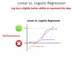
Logistic regression • Suppose we wish look at the proportion of people who give a ‘top box’ score for the satisfaction • Here we have a variable that is binary. Let 0=a 1-4 score and 1 = ‘top box’ or 5 • Natural regression is now logistic as we have binary response • We are now in the wonderful world of generalised linear models
Logistic regression • With Linear regression our mean structure linear depends on the explanatory variables: • m=XTb • With logistic regressionwe have a non-linear response • m=exp(XTb)/(1+ exp(XTb)) • Note that this is a good way of getting around the ‘left skew ness’ of the data
Let’s analyse this data again ## Logistic regression code Regress.eg.logistic.coeff_glm(formula = 1*(Satisfaction==5)~ Straightforward + kept.in.touch + manner.attitude + prompt + fairly, data = Regress.eg, na.action = na.exclude,family=binomial)$coeff
Let’s analyse this data again… > cbind(Regress.eg.coeff, Regress.eg.mlr.coeff[-1], Regress.eg.logistic.coeff[-1]) Straightforward 0.8010022 0.38028138 1.1928456 kept.in.touch 0.7185019 0.16242318 0.6297301 manner.attitude 0.5399704 0.08986848 0.4143086 prompt 0.8653943 0.21992225 1.0494582 fairly 0.6902109 0.15678007 1.0760604 Note that ‘fairly’ comes up as being more important - ie: this is more high associated with top box figures.
More details summary(glm(formula = 1 * (Satisfaction == 5) ~ Straightforward + kept.in.touch + manner.attitude + prompt + fairly, data = Regress.eg, na.action = na.exclude, family = binomial)) Deviance Residuals: Min 1Q Median 3Q Max -2.252605 -0.3172882 0.4059497 0.4059497 2.825783 Coefficients: Value Std. Error t value (Intercept) -19.3572967 1.7395651 -11.127665 Straightforward 1.1928456 0.2674028 4.460857 kept.in.touch 0.6297301 0.2404842 2.618593 manner.attitude 0.4143086 0.1567237 2.643560 prompt 1.0494582 0.2813209 3.730467 fairly 1.0760604 0.2524477 4.262509 (Dispersion Parameter for Binomial family taken to be 1 ) Null Deviance: 744.555 on 545 degrees of freedom Residual Deviance: 358.4669 on 540 degrees of freedom Number of Fisher Scoring Iterations: 5