Finite-Length Scaling and Error Floors
540 likes | 805 Views
Finite-Length Scaling and Error Floors. Tom Richardson. Abdelaziz Amraoui Andrea Montanari Ruediger Urbanke. Approach to Asymptotic. Finite Length Scaling. Finite Length Scaling. Finite Length Scaling. Finite Length Scaling. Analysis (BEC): Covariance evolution.

Finite-Length Scaling and Error Floors
E N D
Presentation Transcript
Finite-Length Scalingand Error Floors Tom Richardson Abdelaziz Amraoui Andrea Montanari Ruediger Urbanke
Analysis (BEC): Covariance evolution Fraction of check nodes of degree greater than one and equal to one. Covariance terms. As a function of residual graph fractional size.
Analysis (BEC) • Follow Luby et al: single variable at a time with the trajectory converging to a differential equation. • Covariance of state space variables also follows a d.e. • Increments have Markov property and regularity.
Generalizing from the BEC? • No obvious incremental form (diff. Eq.) • No state space characterization of failure. • No clear finite dimensional state space. • Not clear what the right coordinates are for the general case (Capacity?). Nevertheless, it is useful in practice to have this interpretation of iterative failure and to have the basic form of the scaling law.
Error floors on the erasure channel: average and typical performance.
Error floors for general channels: Expurgated Ensemble Experiments. Random Girth (8) optimized Neighborhood optimized AWGN channel rate 51/64 block lengths 4k
Error floors for general channels: Trapping set distribution. (3,1) (5,1) (7,1) AWGN channel rate 51/64 block lengths 4k
Observations. • Error floor region dominated by small weight errors. • Subset on which error occur usually induces a subgraph with only degree 2 and degree 1 check nodes where the number of degree 1 check nodes is relatively small. • Optimized graphs exhibit concentration of types of errors.
Nevertheless, if internal received are 1s, internal messaging reaches highly reliable 1 and message state gets trapped. After a few iterations ‘exterior’ nodes and messages converge to high reliability 0s. Internally messages are 1s. In the error floor event, nodes in the trapping sets receive 1’s with some reliability. Other nodes receive typical inputs. (Definite 0) (Reliable 1) 1 1 (Definite 0) (Definite 0) 1 1 1 Intuition (9,3)
Defining Failure: Trapping Sets A decoder on an input ℇYis a sequence of maps: Dl : ℇ {0,1}n (Assume the all-0 codeword is the desired decoding. For the BEC let 1 denote an erasure.) We say that bit j is eventually correct if there exists L so that l > L implies Dl(ℇ) = 0. Assuming failure, the trapping set T is the set of all bits that are not eventually correct.
Defining Failure for BP: Practice Decode for 200 iterations. If the decoding is not successful decode an additional 20 iterations and take the union of all bits that do not decode to 0 during this time.
Trapping Sets: Examples • Let the decoder be the maximum likelihood decoder in one step. Then the trapping sets are the non-zero codewords. • Let the decoder be belief propagation over the BEC. Then the trapping sets are the stopping sets. • Let the decoder be serial (strict) flipping over the BSC. T is a trapping set if and only if the in the subgraph induced by T each node has more even then odd degree neighbors, and the same holds for the complement of T.
Analysis with Trapping Sets:Decomposition of failure FER(s) = T P(ℇT, s) ℇT: The set of all inputs giving rise to failure on trapping set T. Error Floors dominated by “small” events.
Predicting Error Floors: A two pronged attack. • Find (cover) all trapping sets likely to have significant contribution to the error floor region. • T1,T2,T3,….,Tm • Evaluate contribution of each set to the error floor. • P(ℇT1, s), P(ℇT2, s),… Strictly speaking, we get a (tight) lower bound FER(s) > i P(ℇTi, s)
Finding Trapping Sets Simulation of decoding can be viewed as stochastic process for finding trapping sets. It is very inefficient, however. We could use (aided) flipping to get some speed up. It is still too inefficient.
Finding Trapping Sets (Flipping) • Trapping sets can be viewed as “local” extrema of certain functions. E.g., number of odd degree induced checks. • “Local” means, e.g., under single element removal, addition, or swap. Therefore, we can look for subsets that are “local” extrema.
Finding Trapping Sets (Flipping) Basic idea: • Build up a connected subset with bias towards minimizing induced odd degree checks. • Check occasionally for containment of a in-flipping stable set by applying flipping decoding. Eventually such a set is contained. • Check now for other types of variation: • Out-flipping stability. • Single aided flip stability (chains). • ……
Differences: BP and Flipping r1 r2 r1+r2+r3 r3
Evaluating Trapping Sets Basic idea: • Find random variable x on which to condition the decoder input Y that “mostly” determines membership in ℇT. I.e., Pr{ℇT| x}is nearly a step function in x. • Perform in situ simulation of trapping set while varying x to measure Pr{ℇT| x}. • Combine with density of x to get Pr{ℇT}.
Evaluating Trapping Sets Condition input to trapping set Otherwise simulate channel
Evaluating Trapping Sets: BEC X is the number of erasures in T (=S).
Evaluating Trapping Sets: AWGN X is the mean noise input in T.