Download
1 / 58
580 likes | 718 Views
Object Recognition as Machine Translation Matching Words and Pictures. Heather Dunlop 16-721: Advanced Perception April 17, 2006. Machine Translation. Altavista’s Babel Fish: There are three more weeks of classes! Il y a seulement trois semaines supplémentaires de classes!

E N D
Object Recognition as Machine TranslationMatching Words and Pictures Heather Dunlop 16-721: Advanced Perception April 17, 2006
Machine Translation • Altavista’s Babel Fish: • There are three more weeks of classes! • Il y a seulement trois semaines supplémentaires de classes! • ¡Hay solamente tres más semanas de clases! • Ci sono soltanto tre nuove settimane dei codici categoria! • Es gibt nur drei weitere Wochen Kategorien!
Statistical Machine Translation • Statistically link words in one language to words in another • Requires aligned bitext • eg. Hansard for Canadian parliament
Given the translation probabilities, estimate the correspondences Given the correspondences, estimate the translation probabilities Statistical Machine Translation • Assuming an unknown one-one correspondence between words, come up with a joint probability distribution linking words in the two languages • Missing data problem: solution is EM
Multimedia Translation • Data: • Words are associated with images, but correspondences are unknown sun sea sky sun sea sky
Auto-Annotation • Predicting words for the images tiger grass cat
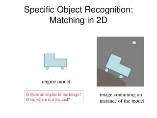
Region Naming • Can also be applied to object recognition • Requires a large data set
Auto-Illustration Moby Dick
Data Sets of Annotated Images • Corel data set • Museum image collections • News photos (with captions)
First Paper Object Recognition as Machine Translation: Learning a Lexicon for a Fixed Image Vocabulary by Pinar Duygulu, Kobus Barnard, Nando de Freitas, David Forsyth • A simple model for annotation and correspondence
Input Representation • Segment with Normalized Cuts: • Only use regions larger than a threshold (typically 5-10 per image) • Form vector representation of each region • Cluster regions with k-means to form blob tokens sun sky waves sea word tokens
Input Representation • Represent each region with a feature vector • Size: portion of the image covered by the region • Position: coordinates of center of mass • Color: avg. and std. dev. of (R,G,B), (L,a,b) and (r=R/(R+G+B),g=G/(R+G+B)) • Texture: avg. and variance of 16 filter responses • Shape: area / perimeter2, moment of inertia, region area / area of convex hull
Assignments • Each word is predicted with some probability by each blob
Expectation Maximization • Select word with highest probability to assign to each blob # of words # of images # of blobs probability that blob bni translates to word wnj probability of obtaining word wnj given instance of blob bni
Given the translation probabilities, estimate the correspondences Given the correspondences, estimate the translation probabilities Expectation Maximization • Initialize to blob-word co-occurrences: • Iterate:
Word Prediction • On a new image: • Segment • For each region: • Extract features • Find the corresponding blob token using nearest neighbor • Use the word posterior probabilities to predict words
Refusing to Predict • Require: p(word|blob) > threshold • ie. Assign a null word to any blob whose best predicted word lies below the threshold • Prunes vocabulary, so fit new lexicon
Indistinguishable Words • Visually indistinguishable: • cat and tiger, train and locomotive • Indistinguishable with our features: • eagle and jet • Entangled correspondence: • polar – bear • mare/foals – horse • Solution: cluster similar words • Obtain similarity matrix • Compare words with symmetrised KL divergence • Apply N-Cuts on matrix to get clusters • Replace word with its cluster label
Experiments • Train with 4500 Corel images • 4-5 words for each image • 371 words in vocabulary • 5-10 regions per image • 500 blobs • Test on 500 images
Auto-Annotation • Determine most likely word for each blob • If probability of word is greater than some threshold, use in annotation
Measuring Performance • Do we predict the right words?
Measuring Performance • Do we predict the right words? • Are they on the right blobs? • Difficult to measure because data set contains no correspondence information • Must be done by hand on a smaller data set • Not practical to count false negatives
Results light bar = average number of times blob predicts word in correct place dark bar = average number of times blob predicts word which is in the image
Second paper Matching Words and Pictures by Kobus Barnard, Pinar Duygulu, Nando de Freitas, David Forsyth, David Blei, Michael I. Jordan • Comparing lots of different models for annotation and correspondence
Annotation Models • Multi-modal hierarchical aspect models • Mixture of multi-modal LDA
Multi-Model Hierarchical Aspect Model cluster = a path from a leaf to the root
observations frequency tables normalization document clusters levels Gaussian Multi-Model Hierarchical Aspect Model • All observations are produced independent of one another • I-0: as above • I-1: cluster dependent level structure • p(l|d) replaced with p(l|c,d) • I-2: generative model • p(l|d) replaced with p(l|c) • allows prediction for documents not in training set
set of observed blobs Multi-Model Hierarchical Aspect Model • Model fitting is done with EM • Word prediction:
mixture component and hidden factor multinomial multinomial Dirichlet multivariate Gaussian multinomial Mixture of Multi-Modal LDA
Mixture of Multi-Modal LDA • Distribution parameters estimated with EM • Word prediction: posterior Dirichlet posterior over mixture components
Correspondence Models • Discrete translation • Hierarchical clustering • Linking word and region emission probabilities • Paired word and region emission
Discrete Translation • Similar to first paper • Use k-means to vector-quantize the set of features representing an image region • Construct a joint probability table linking word tokens to blob tokens • Data set doesn’t provide explicit correspondences • Missing data problem => EM
Hierarchical Clustering • Again, using vector-quantized image regions • Word prediction:
Linking Word andRegion Emission • Words emitted conditioned on observed blobs • D-O: as above (D for dependent) • D-1: cluster dependent level distributions • Replace p(l|c,d) with p(l|d) • D-2: generative model • Replace p(l|d) with p(l) B U W
Paired Word and Region Emission at Nodes • Observed words and regions are emitted in pairs: D={(w,b)} • C-0: as above (C for correspondence) • C-1: cluster dependent level structure • p(l|d) replaced with p(l|c,d) • C-2: generative model • p(l|d) replaced with p(l|c)
Wow, That’s a Lot of models! • Multi-modal hierarchical: I-0, I-1, I-2 • Multi-modal LDA • Discrete translation • Hierarchical clustering • Linked word and region emission: D-0, D-1, D-2 • Paired word and region emission: C-0, C-1, C-2 • Count = 12 • Why so many?
Evaluation Methods • Annotation performance measures: • KL divergence between predicted and target distributions: • Word prediction measure: • n = # of words in image • r = # of words predicted correctly • # of words predicted is set to # of actual keywords • Normalized classification score: • w = # of words predicted incorrectly • N = vocabulary size
Results • Methods using clustering are very reliant on having images that are close to the training data • MoM-LDA has strong resistance to over-fitting • D-0 (linked word and region emission) appears to give best results, taking all measures and data sets into consideration
Unsuccessful Results good annotation, poor correspondence complete failure