Download
1 / 27
270 likes | 287 Views
Learn about mathematical modelling, constitutive equations, and physical properties of mechanically incompressible, thermally expansible viscous fluids in this comprehensive lecture series.

E N D
Flow of mechanically incompressible, but thermally expnsible viscous fluids A. Mikelic, A. Fasano, A. Farina Montecatini, Sept. 9 - 17
LECTURE 1. • Basic mathemathical modelling • LECTURE 2. • Mathematical problem • LECTURE 3. • Stability
Definitions and basic equations We start by recalling the mass balance, the momentum and energy equations, as well as the Clausius-Duhem inequality in the Eulerian formalism. Following an approach similar to the one presented in [1], pages 51-85, we denote by: the density, velocity, specific internal energy, absolute temperature and specific entropy, satisfying the following system of equations: [1]. H. Schlichting, K. Gersten, Boundary-Layer Theory, 8th edition, Springer, Heidelberg, 2000.
where: • denotes the material derivative. • is the rate of strain tensor. • T is the Cauchy stress tensor. Further, • is the heat flux vector. • is the gravity acceleration. Indeed is the unit vector relative to the x3 • axis directed upward. • In the energy equation the internal heat sources are disregarded.
Introducing the specific (i.e. per unit mass) Helmholtz free energy and using the energy equation, Clausius-Duhem inequality becomes
Constitutive equations Key point of the model is to select suitable constitutive equations for in terms of the dependent variables The constitutive equations selection has to be operated considering the physicalproperties of the fluids we dial with.
Main physical properties • The fluid is mechanically incompressible butthermally • dilatable(i.e. the fluid can sustain only isochoric motion in • isothermal conditions) T 1 T 2 > T1 • The fluidbehaves as a linear viscous fluid (Newtonian fluid) Shear stress proportional to shear rate
Vin , Tin Vfin , Tfin thermal expansion coefficient We assume that b may depend on temperature, but not on pressure, i.e.
^ in general we have r = r ( T ) r function of temperature So, if, for instance, b is constant,
Vin , Tin Vfin , Tfin refernce configuration actual configuration i.e. J is a function of T, and can be expressed in terms of the thermal expansion coeff. b
Since J=J(T), continity equation reads as a constraint linking temperature variations with the divergence of the velocity field.
If T is uniform and constant the flow is isochoric Remark First consequence of our modelling: We have introduced a CONSTRAINT. The admissible flows are those that fulfill the condition force that maintains the constraint
rigid box fluid T = 0° C Physical remark The constraint r = r ( T ) models the fluid as being incompressible under isothermal conditions, but whose density changes in response to changes in temperature. In other words, given a temperature T the fluid is capable to exert any forcefor reaching the corresponding density. T = 20° C The box brakes According to the model T = 20° C The box does not brake According to the reality
Let us now turn to a discussion of the constraint. We start considering the usual incompressibility constraint We proceed applying classical procedure. We modify the forces by adding, as in classical mechanics, a term(the socalled constraint response) due to the constraint itself. We thus consider • Where the subscript rindicates the portion of the stress given by • constitutive equations and subscript crefers to the constraint response. • The contraint response is required: • to have no dependendance on the state variables • to produce no entropy in any motion that satisfies the constarint, i.e.
Hece, the above conditions demand that: 1. There is no constitutive equation for p, i.e. p does not depend on any variable defining the state of the system. p, usually referred to as mechanical pressure, is a new state variable of the system. 2.
Fc Fc dx dx Remark Smooth constraints in classical mechanics (D'Alembert ) Constarint response Displacement compatible with the constraint
In the general case (density-temperature constraint, for instance) it is assumed that the dependent quantities are determined by constitutive functions only up to an additive constraint response (see [2], [3]) r constitutive, c constraint The contraint responses are required to do not dissipate energy Recalling [2] Adkins, 1958 [3] Green, Naghdi, Trapp, 1970
no entropy production, i.e. no dissipation we have (1) when T and are such that Considering various special subsets of the set of all allowable thermomechanical processes, the above equation leads to
Hence Where p is a function of position and time. Recall: There is no constitutive quation for p. The function p defined above is usually referred to as mechanical pressure and is not the thermodynamic pressure that is defined through an equation of state.
Remark 1 There is also another formulation of the theory. We briefly summarize it We start considering the theory of a compressible (i.e. unconstrained) fluid, introducing the Helmholtz free energy • and we develop the standard theory considering which • gives . We deduce that: • There is no equation of state defining the pressure p. The distinctions of the two constraint theory approaches are as follows: The first approach assumes the existence of an additive constraint response, postulated to produce no entropy, whereas the above approach deduces the additive constraint response.
Remark 2 • Constraints that are nonlinear cannot, in general, be considered by the • Procedure prevuously illustrated. • For example, consider this constraint(1) • Now the conditions to be imposed are: • whenever • does not depend on the state variables • We can nolonger demand that condition 2 is fulfilled !! (1) Such a constraint is for illustrative purposes only and does not necessarily correspond to a physically meaningful situation.
Deduction of the constitutive equations Assumption 1. Assumption 2. Linear viscous fluid Setting so that we have
So, we are left with and assume OK !!
ASSUMTION Summarizing
Remark Informulating constitutive models, such as, for instance, y=y(T),we must have in mind some inferential method for quantifying them. Concerning y(T ) we shall return to this point later.