Download
1 / 47
470 likes | 535 Views
This resource covers different aspects of load balancing in parallel computers, including reasons for inefficiencies, measuring load imbalance, graph partitioning, spectra of solutions, and dynamic load balancing methods. It also delves into search problems, tree search examples, and optimization strategies. Discover when to use static, semi-static, or dynamic load balancing and what differentiates each approach. Learn about tools like TAU for measuring load imbalance and optimizing parallel computations.

E N D
CS 267: Applications of Parallel ComputersLoad Balancing James Demmel www.cs.berkeley.edu/~demmel/cs267_Spr10 CS267 Lecture 23
Outline • Motivation for Load Balancing • Recall graph partitioning as load balancing technique • Overview of load balancing problems, as determined by • Task costs • Task dependencies • Locality needs • Spectrum of solutions • Static - all information available before starting • Semi-Static - some info before starting • Dynamic - little or no info before starting • Survey of solutions • How each one works • Theoretical bounds, if any • When to use it, tools CS267 Lecture 23
Sources of inefficiency in parallel codes • Poor single processor performance • Typically in the memory system (recall matmul homework) • Too much parallelism overhead • Thread creation, synchronization, communication • Load imbalance • Different amounts of work across processors • Computation and communication • Different speeds (or available resources) for the processors • Possibly due to load on shared machine • How to recognize load imbalance • Time spent at synchronization is high and is uneven across processors, but not always so simple … CS267 Lecture 23
Measuring Load Imbalance • Challenges: • Can be hard to separate from high synchronization overhead • Especially subtle if not bulk-synchronous • “Spin locks” can make synchronization look like useful work • Note that imbalance may change over phases • Insufficient parallelism always leads to load imbalance • Tools like TAU can help (acts.nersc.gov) CS267 Lecture 23
Review of Graph Partitioning • Partition G(N,E) so that • N = N1 U … U Np, with each |Ni| ~ |N|/p • As few edges connecting different Ni and Nk as possible • If N = {tasks}, each unit cost, edge e=(i,j) means task i has to communicate with task j, then partitioning means • balancing the load, i.e. each |Ni| ~ |N|/p • minimizing communication volume • Optimal graph partitioning is NP complete, so we use heuristics (see earlier lectures) • Spectral, Kernighan-Lin, Multilevel … • Good software available • (Par)METIS, Zoltan, … • Speed of partitioner trades off with quality of partition • Better load balance costs more; may or may not be worth it • Need to know tasks, communication pattern before starting • What if you don’t? Can redo partitioning, but not frequently CS267 Lecture 23
Load Balancing Overview Load balancing differs with properties of the tasks (chunks of work): • Tasks costs • Do all tasks have equal costs? • If not, when are the costs known? • Before starting, when task created, or only when task ends • Task dependencies • Can all tasks be run in any order (including parallel)? • If not, when are the dependencies known? • Before starting, when task created, or only when task ends • One task may prematurely end another task • Locality • Is it important for some tasks to be scheduled on the same processor (or nearby) to reduce communication cost? • When is the information about communication known? CS267 Lecture 23
, search Task Cost Spectrum CS267 Lecture 23
Task Dependency Spectrum CS267 Lecture 23
Task Locality Spectrum (Communication) CS267 Lecture 23
Spectrum of Solutions A key question is when certain information about the load balancing problem is known. Leads to a spectrum of solutions: • Static scheduling. All information is available to scheduling algorithm, which runs before any real computation starts. • Off-line algorithms, eg graph partitioning, DAG scheduling • Semi-static scheduling. Information may be known at program startup, or the beginning of each timestep, or at other well-defined points. Offline algorithms may be used even though the problem is dynamic. • eg Kernighan-Lin, as in Zoltan • Dynamic scheduling. Information is not known until mid-execution. • On-line algorithms – main topic today CS267 Lecture 23
Dynamic Load Balancing • Motivation for dynamic load balancing • Search algorithms as driving example • Centralized load balancing • Overview • Special case for schedule independent loop iterations • Distributed load balancing • Overview • Engineering • Theoretical results • Example scheduling problem: mixed parallelism • Demonstrate use of coarse performance models CS267 Lecture 23
Search • Search problems are often: • Computationally expensive • Have very different parallelization strategies than physical simulations. • Require dynamic load balancing • Examples: • Optimal layout of VLSI chips • Robot motion planning • Chess and other games (N-queens) • Speech processing • Constructing phylogeny tree from set of genes CS267 Lecture 23
Example Problem: Tree Search • In Tree Search the tree unfolds dynamically • May be a graph if there are common sub-problems along different paths • Graphs unlike meshes which are precomputed and have no ordering constraints Terminal node (non-goal) Non-terminal node Terminal node (goal) CS267 Lecture 23
Depth vs Breadth First Search (Review) • DFS with Explicit Stack • Put root into Stack • Stack is data structure where items added to and removed from the top only • While Stack not empty • If node on top of Stack satisfies goal of search, return result, else • Mark node on top of Stack as “searched” • If top of Stack has an unsearched child, put child on top of Stack, else remove top of Stack • BFS with Explicit Queue • Put root into Queue • Queue is data structure where items added to end, removed from front • While Queue not empty • If node at front of Queue satisfies goal of search, return result, else • Mark node at front of Queue as “searched” • If node at front of Queue has any unsearched children, put them all at end of Queue • Remove node at front from Queue CS267 Lecture 23
Sequential Search Algorithms • Depth-first search (DFS) • Simple backtracking • Search to bottom, backing up to last choice if necessary • Depth-first branch-and-bound • Keep track of best solution so far (“bound”) • Cut off sub-trees that are guaranteed to be worse than bound • Iterative Deepening • Choose a bound d on search depth, and use DFS up to depth d • If no solution is found, increase d and start again • Can use an estimate of cost-to-solution to get bound on d • Breadth-first search (BFS) • Search all nodes at distance 1 from the root, then distance 2, and so on CS267 Lecture 23
Load balance on 2 processors Load balance on 4 processors Parallel Search • Consider simple backtracking search • Try static load balancing: spawn each new task on an idle processor, until all have a subtree • We can and should do better than this … CS267 Lecture 23
Centralized Scheduling • Keep a queue of task waiting to be done • May be done by manager task • Or a shared data structure protected by locks worker worker Task Queue worker worker worker worker CS267 Lecture 23
Centralized Task Queue: Scheduling Loops • When applied to loops, often called self scheduling: • Tasks may be range of loop indices to compute • Assumes independent iterations • Loop body has unpredictable time (branches) or the problem is not interesting • Originally designed for: • Scheduling loops by compiler (or runtime-system) • Original paper by Tang and Yew, ICPP 1986 • Properties • Dynamic, online scheduling algorithm • Good for a small number of processors (centralized) • Special case of task graph – independent tasks, known at once CS267 Lecture 23
Variations on Self-Scheduling • Typically, don’t want to grab smallest unit of parallel work, e.g., a single iteration • Too much contention at shared queue • Instead, choose a chunk of tasks of size K. • If K is large, access overhead for task queue is small • If K is small, we are likely to have even finish times (load balance) • (at least) Four Variations: • Use a fixed chunk size • Guided self-scheduling • Tapering • Weighted Factoring CS267 Lecture 23
Variation 1: Fixed Chunk Size • Kruskal and Weiss give a technique for computing the optimal chunk size (IEEE Trans. Software Eng., 1985) • Requires a lot of information about the problem characteristics • e.g., task costs, number of tasks, cost of scheduling • Probability distribution of runtime of each task (same for all) • Not very useful in practice • Task costs must be known at loop startup time • E.g., in compiler, all branches be predicted based on loop indices and used for task cost estimates CS267 Lecture 23
Variation 2: Guided Self-Scheduling • Idea: use larger chunks at the beginning to avoid excessive overhead and smaller chunks near the end to even out the finish times. • The chunk size Ki at the ith access to the task pool is given by Ki = ceiling(Ri/p) • where Ri is the total number of tasks remaining and • p is the number of processors • See Polychronopolous, “Guided Self-Scheduling: A Practical Scheduling Scheme for Parallel Supercomputers,” IEEE Transactions on Computers, Dec. 1987. CS267 Lecture 23
Variation 3: Tapering • Idea: the chunk size, Ki is a function of not only the remaining work, but also the task cost variance • variance is estimated using history information • high variance => small chunk size should be used • low variance => larger chunks OK • See S. Lucco, “Adaptive Parallel Programs,” PhD Thesis, UCB, CSD-95-864, 1994. • Gives analysis (based on workload distribution) • Also gives experimental results -- tapering always works at least as well as GSS, although difference is often small CS267 Lecture 23
Variation 4: Weighted Factoring • Idea: similar to self-scheduling, but divide task cost by computational power of requesting node • Useful for heterogeneous systems • Also useful for shared resource clusters, e.g., built using all the machines in a building • as with Tapering, historical information is used to predict future speed • “speed” may depend on the other loads currently on a given processor • See Hummel, Schmit, Uma, and Wein, SPAA ‘96 • includes experimental data and analysis CS267 Lecture 23
When is Self-Scheduling a Good Idea? Useful when: • A batch (or set) of tasks without dependencies • can also be used with dependencies, but most analysis has only been done for task sets without dependencies • The cost of each task is unknown • Locality is not important • Shared memory machine, or at least number of processors is small – centralization is OK CS267 Lecture 23
Distributed Task Queues • The obvious extension of task queue to distributed memory is: • a distributed task queue (or “bag”) • Idle processors can “pull” work, or busy processors “push” work • When are these a good idea? • Distributed memory multiprocessors • Or, shared memory with significant synchronization overhead • Locality is not (very) important • Tasks may be: • known in advance, e.g., a bag of independent ones • dependencies exist, i.e., being computed on the fly • The costs of tasks is not known in advance CS267 Lecture 23
Distributed Dynamic Load Balancing • Dynamic load balancing algorithms go by other names: • Work stealing, work crews, … • Basic idea, when applied to tree search: • Each processor performs search on disjoint part of tree • When finished, get work from a processor that is still busy • Requires asynchronous communication busy idle Service pending messages Select a processor and request work No work found Do fixed amount of work Service pending messages Got work CS267 Lecture 23
How to Select a Donor Processor • Three basic techniques: • Asynchronous round robin • Each processor k, keeps a variable “targetk” • When a processor runs out of work, requests work from targetk • Set targetk= (targetk +1) mod procs • Global round robin • Proc 0 keeps a single variable “target” • When a processor needs work, gets target, requests work from target • Proc 0 sets target = (target + 1) mod procs • Random polling/stealing • When a processor needs work, select a random processor and request work from it • Repeat if no work is found CS267 Lecture 23
How to Split Work • First parameter is number of tasks to split • Related to the self-scheduling variations, but total number of tasks is now unknown • Second question is which one(s) • Send tasks near the bottom of the stack (oldest) • Execute from the top (most recent) • May be able to do better with information about task costs Top of stack Bottom of stack CS267 Lecture 23
Theoretical Results (1) Main result: Simple randomized algorithms are optimal with high probability • Karp and Zhang [88] show this for a tree of unit cost (equal size) tasks • Parent must be done before children • Tree unfolds at runtime • Task number/priorities not known a priori • Children “pushed” to random processors • Show this for independent, equal sized tasks • “Throw n balls into n random bins”: Q ( log n / log log n ) in fullest bin • Throw d times and pick the emptiest bin: log log n / log d [Azar] • Extension to parallel throwing [Adler et all 95] • Shows p log p tasks leads to “good” balance CS267 Lecture 23
Theoretical Results (2) Main result: Simple randomized algorithms are optimal with high probability • Blumofe and Leiserson [94] show this for a fixed task tree of variable cost tasks • their algorithm uses task pulling (stealing) instead of pushing, which is good for locality • I.e., when a processor becomes idle, it steals from a random processor • also have (loose) bounds on the total memory required • Used in Cilk • Chakrabarti et al [94] show this for a dynamic tree of variable cost tasks • works for branch and bound, i.e. tree structure can depend on execution order • uses randomized pushing of tasks instead of pulling, so worse locality • Open problem: does task pulling provably work well for dynamic trees? CS267 Lecture 23
Distributed Task Queue References • Introduction to Parallel Computing by Kumar et al (text) • Multipol library (See C.-P. Wen, UCB PhD, 1996.) • Part of Multipol (www.cs.berkeley.edu/projects/multipol) • Try to push tasks with high ratio of cost to compute/cost to push • Ex: for matmul, ratio = 2n3 cost(flop) / 2n2 cost(send a word) • Goldstein, Rogers, Grunwald, and others (independent work) have all shown • advantages of integrating into the language framework • very lightweight thread creation • CILK (Leiserson et al) (supertech.lcs.mit.edu/cilk) • Recently acquired by Intel CS267 Lecture 23
Diffusion-Based Load Balancing • In the randomized schemes, the machine is treated as fully-connected. • Diffusion-based load balancing takes topology into account • Send some extra work to a few nearby processors • Analogy to diffusion • Locality properties better than choosing random processor • Load balancing somewhat slower than randomized • Cost of tasks must be known at creation time • No dependencies between tasks CS267 Lecture 23
Diffusion-based load balancing • The machine is modeled as a graph • At each step, we compute the weight of task remaining on each processor • This is simply the number if they are unit cost tasks • Each processor compares its weight with its neighbors and performs some averaging • Analysis using Markov chains • See Ghosh et al, SPAA96 for a second order diffusive load balancing algorithm • takes into account amount of work sent last time • avoids some oscillation of first order schemes • Note: locality is still not a major concern, although balancing with neighbors may be better than random CS267 Lecture 23
Mixed Parallelism As another variation, consider a problem with 2 levels of parallelism • course-grained task parallelism • good when many tasks, bad if few • fine-grained data parallelism • good when much parallelism within a task, bad if little Appears in: • Adaptive mesh refinement • Discrete event simulation, e.g., circuit simulation • Database query processing • Sparse matrix direct solvers How do we schedule both kinds of parallelism well? CS267 Lecture 23
Mixed Parallelism Strategies CS267 Lecture 23
Which Strategy to Use More data, less task parallelism More task, less data parallelism And easier to implement CS267 Lecture 23
Switch Parallelism: A Special Case See Soumen Chakrabarti’s 1996 UCB EECS PhD Thesis See also J. Parallel & Distributed Comp, v. 47, pp 168-184, 1997 CS267 Lecture 23
Extra Slides CS267 Lecture 23
Simple Performance Model for Data Parallelism CS267 Lecture 22
Modeling Performance • To predict performance, make assumptions about task tree • complete tree with branching factor d>= 2 • d child tasks of parent of size N are all of size N/c, c>1 • work to do task of size N is O(Na), a>= 1 • Example: Sign function based eigenvalue routine • d=2, c=2 (on average), a=3 • Combine these assumptions with model of data parallelism CS267 Lecture 22
Actual Speed of Sign Function Eigensolver • Starred lines are optimal mixed parallelism • Solid lines are data parallelism • Dashed lines are switched parallelism • Intel Paragon, built on ScaLAPACK • Switched parallelism worthwhile! CS267 Lecture 22
Values of Sigma (Problem Size for Half Peak) CS267 Lecture 22
Best-First Search • Rather than searching to the bottom, keep set of current states in the space • Pick the “best” one (by some heuristic) for the next step • Use lower bound l(x) as heuristic • l(x) = g(x) + h(x) • g(x) is the cost of reaching the current state • h(x) is a heuristic for the cost of reaching the goal • Choose h(x) to be a lower bound on actual cost • E.g., h(x) might be sum of number of moves for each piece in game problem to reach a solution (ignoring other pieces) CS267 Lecture 22
Branch and Bound Search Revisited • The load balancing algorithms as described were for full depth-first search • For most real problems, the search is bounded • Current bound (e.g., best solution so far) logically shared • For large-scale machines, may be replicated • All processors need not always agree on bounds • Big savings in practice • Trade-off between • Work spent updating bound • Time wasted search unnecessary part of the space CS267 Lecture 22
Simulated Efficiency of Eigensolver • Starred lines are optimal mixed parallelism • Solid lines are data parallelism • Dashed lines are switched parallelism CS267 Lecture 22
Simulated efficiency of Sparse Cholesky • Starred lines are optimal mixed parallelism • Solid lines are data parallelism • Dashed lines are switched parallelism CS267 Lecture 22