II-6 Stellar Mass and Binary Stars (Main Ref.: Lecture notes;

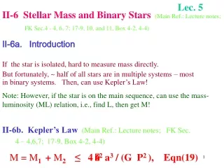
Lec. 5 II-6 Stellar Mass and Binary Stars(Main Ref.: Lecture notes; FK Sec.4 - 4, 6, 7; 17-9, 10, and 11, Box 4-2, 4-4) II-6a. Introduction If the star is isolated, hard to measure mass directly. But fortunately, ~ half of all stars are in multiple systems – most in binary systems. Then, can use Kepler’s Law! Note: However, if the star is on the main sequence, can use the mass-luminosity (ML) relation, i.e., find L, then get M! II-6b. Kepler’s Law(Main Ref.: Lecture notes; FK Sec. 4 – 4,6,7; 17-9, Box 4-2, 4-4) M = M1 + M2 ≤ 4 2 a3 / (G P2 ), Eqn(19)

where M1, M2 are mass of Star 1 and Star 2; P = orbital period; a = separation between Star 1 and Star 2 = semi-major axis of one star’s orbit around another. G = 6.67 x 10–11 Newton m2 /kg2 = Universal constant of gravitation. Often elliptical orbit (see Fig. II-31a, 31b), but for simplicity, we will assume a circular orbit. Fig II-31a: A Binary Star System

Note: the (=) sign only if the inclination angle  of the orbital plane to the plane of the sky is known. If not, the (<) sign applies, i.e., only the maximum mass of the system M will be found. Note: in Fig. II-32, M1 < M2 (See class notes for explanation.) Fig II-31b: Elliptical Orbit M2 2 M1 1 a2 a1 COM x a Fig II-32: Binary System

Center of Mass (COM): In the case of two stars in a binary system, Star 1 and Star 2 move about COM. See FK for more general definition. See Fig. II-32 and 33. Fig II-33: Center of Mass

Often orbit is elliptical (e.g., see Fig. II-31a, 31b), but for simplicity here we assume the orbit is circular. Note: From mechanics and the definition of COM - see Fig. II-32, a1 M1 = a2 M2 Eqn(20a) a = a1 + a2 Eqn(20b) where a1 and a2 are the distance of Star 1 and Star 2 from COM. Now, use special unit: then, M1 + M2 ≤ a3 / P2 Eqn(21a) M = M1 + M2 Eqn(21b) when M, M1 and M2 in unit of M(solar), P in year, and a in AU. M = total mass of the system. See Section II-6e for examples.

II-6c. Binary Stars(Main Ref.: Lecture notes; FK Sec. 5-9, 17-9, 17-10, 17-11) (i) Visual Binaries (FK Sec. 17-9, Lecture notes) Can visually resolve the two component stars of the binary. Some coincidence (called `optical double stars’) and the two stars are not related. But most of them are real double stars – i.e., gravitationally bound binary, moving around the COM. (ii) Spectrum Binaries (FK Sec. 17-10, Lecture notes) Binary consists of two stars of different spectral types. Although two stars cannot be visually resolved separately (too far from us, too close to each other, or both), we can identify the two stars by the presence of two different classes of spectral lines.

(iii) Spectroscopic Binaries (FK Sec. 5-9, 17-10, Lecture notes) We can identify the binary motion, characteristics of the component stars, etc., by measuring periodic shifting of spectral lines due to the Doppler effect as the stars move around the COM. In most cases the component two stars cannot be visually resolved separately, however (too far from us, too close to each other, or both). In some cases, the shifting of spectral lines can be resolved for both stars. In many cases the shifts can be resolved for only one of the stars – e.g., because the line is too weak, or shift too small. See class notes and Fig. II-34 and 35 (next page) for the detailed explanation.

Fig II-34 Radial Velocity Curves Fig II-35 Shift of Spectral Lines

Doppler Effect:See FK Sec. 5-9, Lecture notes  / 0 = ( – 0) / 0 = v/ c Eqn(22) (non-rel.) Also, (v1 / v2 ) = (a1 / a2 ) Eqn(23a) v = radial velocity. (Derivation not given in this class.) v = v1 + v2 = 2 π a / P Eqn(23b) v1,2 = 2 π a1,2 / P Eqn(23b) Method: From the observation and analysis of the spectrum such as Fig. II-35, measure P, 1, 1, 2 and 2. 1, 1, 2 and 2 Eqn(22) for Star 1 and Star 2 separately(*)  get v1 and v2  get (v1 / v2 ). Then, solve Eqns (20a), (20b), (21a), (21b) and (23), and we can find M1 and M2 separately (see EX. 26). (*) If the lines of only one of the two stars are strong enough for the above analysis, we do not get M1 and M2 separately.

Inclination Angle  - complication The above analysis applies if we are looking edge on (for spectroscopic binaries). Normally it is not. Then, only the maximum mass known. (See class notes for the explanation.) If the binary is also an eclipsing or visual binary, we can often find . Then, can find real mass, not maximum mass(not required for this course – discussed in Physics 435.) (iv) Eclipsing Binaries (FK Sec. 17-11, Lecture notes) When one star of a binary gets behind the other star, eclipse happens. The intensity (brightness) of the binary vs time curve is called `light curve’. Then the shape of the light curve can often determine various useful parameters, e.g., the inclination angle , nature of the stellar atmosphere, and sometimes even stellar radius. See class notes and Fig. II-36 for explanation.

Fig II-36: Eclipsing Binaries

II-6d. Mass Luminosity Relation(Main Ref.: Lecture notes; FK Sec.17-9) For main sequence stars (only!), stellar luminosity L and mass M are related by: L ~ a M4(*) Eqn (24a) a is some constant. Derivation in Physics 435, but not in this course. (*) Note: it deviates from 4 for both low and high mass, but ~ o.k. See Fig. II-37. By dividing Eqn (24a) for the star by that for the sun, we get: L / L☉ ~ ( M / M☉)4 Eqn (24b) ********************************************** EX 23 1 M☉ Star  ~ 1 L☉; 10 M☉ Star  ~ 104L☉; 0.1 M☉ Star  ~ 10-4L☉

Note: ms mass changes from ~ 0.2  60 M☉. FK FK Fig II-37 Mass Luminosity Relation Fig II-38 Mass on the H-R Diagram

II-6e. Examples EX 24 Two stars in a binary system have the same mass of 2M☉ and they are separated by 4 AU. What is the orbital period? Ans: 4 years.(see class notes.) ************************************************************************************* EX 25 Two stars in a binary system are separated by 4 AU and their orbital period is 1 year. What is the total mass of the system? Ans: 64 M☉.(see class notes.) ************************************************************************************* EX 26 In problem EX 25, the ratio of the distance of Star 1 from COM to that of Star 2 is 3. What are the mass and distance from COM of Star 1 and Star 2? Ans: Star 1 is 16 M☉, and Star 2 is 48 M☉. Distance of Star 1 and 2 from COM are 3AU and 1AU, respectively. (See class notes.)

How to find Mass? (Summary) • If stars are in a binary system, use Kepler’s Law ((Eqn(19) or Eqns(21a)(21b))  If we can measure a and P, we get the total mass of the system M. P can be measured directly for all binary kinds if it is not too long. a can be measured if the system is looked edge on (both for spectroscopic and eclipsing binaries) or if inclination angle is found (o.k. for some visual and eclipsing binaries). Otherwise, only the maximum mass can be found. • If both a1 and a2 (or their ratio a1/a2) are found (can happen for some of all binary kinds), then Eqns (20a)(20b) give mass of both stars separately. • If it is a spectroscopic binary, the relative wavelength shifts of the lines of the two stars (if both can be resolved) will give ratio of the radial velocity of the two stars, which gives the ratio a1/a2 from Eqn(23). • If a star is a main sequence star, the mass luminosity relation Eqn(24b) and measurement of luminosity give mass.

II-7 Stellar Structure and Energy Source (Main Ref.: Lecture notes; FK Sec. 16-1, 16-2) II-7a. Energy Source for Main Sequence Stars (Main Ref.: Lecture notes; FK Sec.16-1) Gravitational Source:too fast! tG = 2.5 x 106 years! But: geological and biological evidence, radioactive decay time, etc.  Age of the Earth t~ 4.6 x 109 years ~ Age of the sun t☉. So,  Sun must be as old! Chemical Source:even faster! tC ~ 104 years! Nuclear Source:o.k.! tN ~ 1010 years! Nuclear Fusion: Main Sequence stars  4 H  He + energy Eqn(25)

Low mass stars pp chain, high mass stars CNO cycle (details not required for this class). Idea: Mass m can be converted to energy E, by Einstein’s: E = m c2 Eqn(26) By the `Hydrogen (H)-Burning’ (i.e., H  He conversion = Eqn(25)), 0.7 % of total stellar mass will be converted to energy (Derivation optional) But H-burning stops in the central region of the star when ~ 10  30% of the mass changes from H to He (see Sections II-7b and 8b). Then, we get: duration of H-burning =tN ~ 1010 years! Derivation: use Eqn(26) and relation EN ~ L☉ tN ~ m c2. Eqn(27) EN = nuclear energy released by H-burning. m is the fraction of stellar mass converted to energy by H-burning = 0.007 x (0.1 – 0.3) M☉. See HW V-4 and class notes for the details. Note: 1 year ~ 3 x 107 sec., c = 3 x 108 m/sec, L☉ = 4 x 1026 J/sec., M☉= 1.9891 x 1030 kg

II-7b. Stellar Structure-Models (Main Ref.: Lecture notes; FK Sec.16-2) Stellar interior – hot, e.g., central core temperature Tc≥ ~ 107 K for stars like the sun (- compare with the surface temperature Ts = 5800 K). H and He (main composition) all ionized at such high T. Note: Thermonuclear reactions (e.g., H-burning) take place only in the central high T core. Stellar structure found by solving basic stellar structure equations: (i) Hydrostatic Equilibrium: mecahnical balance, (ii) Energy Balance: Total energy production/sec = Total energy loss/sec,

(iii) Energy Transport: the manner in which energy produced in the central core is transported to the surface. (iiia) Conduction: energy carried by free electrons (e.g., metals). (iiib) Radiation: energy carried by photons (`random walk’ – takes long time from interior to surface). (iiic) Convection: energy carried by particles, by gas motion (e.g. boiling watter). • By solving these basic equations, can find the stellar structure  • Results: see Fig. II-40, 41. Note: Temperature T, pressure P and density  decrease, while luminosity L and mass m increase, from center to surface. Note: T > ~ 107 K only for r < 0.20 R☉, where H-burning can take place. (See class notes for detailed explanation.)

Fig II-39: Pressure Balance Fig II-40: Sun’s Interior Structure Table II-4: Model of Solar Structure

Fig II-41: Interior Structure of a Sun-like Star – radial distribution of L, m, T, and .

II-6 Stellar Mass and Binary Stars (Main Ref.: Lecture notes;