Spectral Characteristics of Convective-Scale Precipitation Observations and Forecasts

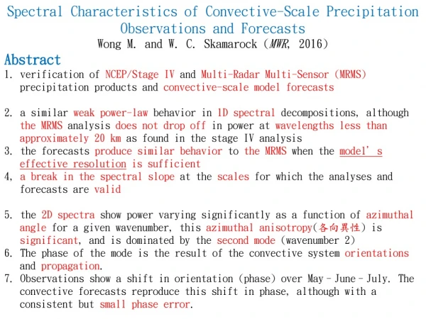
1. Spectral Characteristics of Convective-Scale Precipitation Observations and Forecasts Wong M. and W. C. Skamarock (MWR, 2016) Abstract 1. verification of NCEP/Stage IV and Multi-Radar Multi-Sensor (MRMS) precipitation products and convective-scale model forecasts 2. a similar weak power-law behavior in 1D spectraldecompositions, although the MRMS analysis does not drop off in power at wavelengths less than approximately 20 km as found in the stage IV analysis 3. the forecasts produce similar behavior to the MRMS when the model’s effective resolution is sufficient 4, a break in the spectral slope at the scales for which the analyses and forecasts are valid 5. the 2D spectrashow power varying significantly as a function of azimuthal angle for a given wavenumber, this azimuthal anisotropy(各向異性) is significant, and is dominated by the second mode (wavenumber 2) 6. The phase of the mode is the result of the convective system orientations and propagation. 7. Observations show a shift in orientation (phase) over May–June–July. The convective forecasts reproduce this shift in phase, although with a consistent but small phase error.

2. 1. Introduction (general) 1. convection-permitting forecast models: horizontal spacing of a few km or less deep convective updrafts are explicitly simulated produce convective-system structure and evolution very similar to obs. allow for better representation of terrain and topographic flow effects 2. Traditional approaches for comparing precipitation forecasts to obs. such as ETS and bias do not provide any direct measure of the scale or structure of precipitation features. 3. Scaleis an important consideration in forecast model performance; specifically, what scales are resolved in a model forecast, and are they resolved properly.

3. 1. Introduction (1D & 2D spectra) 4. Observational analyses using 1D spectra exhibit a power-law relationship for precipitation as a function of horizontal scale, and this relationship is consistent with the power-law relationship observed for the horizontal wind fields, specifically the kinetic energy. 5. The 1D spectral analyses: 1) do observations show any breakin the power-law scaling and 2) do convection permitting model forecasts reproduce the power-law scaling, and over what scales are the forecast spectra accurate? 6. The smallest scale where observed power-law scaling holds is one definition of the effective resolution of a model configuration, usually evaluated using horizontal or vertical velocity spectra. 7. The 2D precipitation spectra are cast in polar coordinates (horizontal wavenumber, azimuth) and the characteristics of the spectra as a function of azimuth for a given wavelength are examined. 8. Examined how the variance and structure of the precipitation fields evolve from late spring (May) through summer (July). The observed 2D precipitation spectra change noticeably over the 2.5-month period, and this change is also evident in the forecast spectra.

4. 2. Description of models and observations 1. Temporally averaged vertical velocity, horizontal kinetic energy, and precipitation spectra are computed from hourly forecastsand precipitation analyses over a domain with 720×720 grid points (1800×1800 points for the MRMS analyses). The MPAS and NCEP/stageIV are interpolated to a 0.025°× 0.025° grid, the MRMS are on a 0.01°× 0.01° grid. 2. case study: WRF 3-km (0.025°) WRF 1-km (0.01°)

5. 2. Description of models and observations 3. Two sets of MPAS: [lacking 1~7 June??] a. NOAA Hazardous Weather Testbed (HWT) between 1 and 31 May, daily 5-day (120 h) forecasts, initialized by the 0000 UTC Global Forecast System (GFS) analysis b. Plains Elevated Convection At Night (PECAN) between 8 June and 14 July, 3-day (72 h) forecasts, initialized by the 0000 UTC GFS analysis nominally 3-km horizontal grid spacing MYNN surface layer scheme and planetary boundary layer (PBL) scheme the Grell-Freitas scale-aware cumulus scheme the WSM6 single-moment microphysics scheme the Rapid Radiative Transfer Model for GCM (RRTMG) short- and longwave radiation schemes

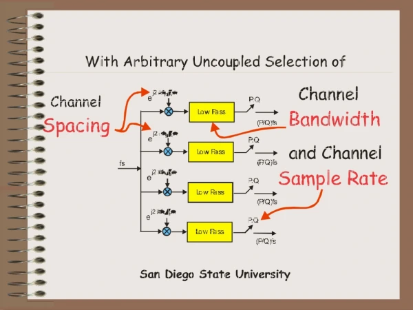
6. Model for Prediction Across Scales (https://mpas-dev.github.io) 1. Global model 2. Voronoi (hexagonal) meshes (沃羅諾伊空間分割) and C-grid staggering

7. 2. Description of models and observations 4. NCEP/stage IV 4-km gridded precip. estimates: (Lin & Mitchell 2005) regional hourly and 6-hourly based on WSR-88D observations bias corrected using rain gauge measurements and satelliteinformation some manual quality control by forecasters 5. MRMS 1-km gridded precipitation estimates: (Zhang et al. 2014, 2016) (regional) hourly combining information from multiple radars in the United States and Canada, lightning and rain gauges, climatology data, satellite data, atmospheric environmental data, and NWP model output. fully automated and do not benefit from manual quality control

8. 2. Description of models and observations 6. To avoid model spinuperrors, such as that discussed in Skamarock (2004), we do not use the first 24 forecast hours in our spectral calculations. 7. MPAS typically overestimates the diurnal precipitation maximumand underestimates the minimum, but the model bias does not vary significantlywith forecast lead time. [10% differences between MRMS and Stage IV??] [spinup 10 h??] [what fcst data selected??]

9. 2. Description of models and observations 8. case study: WRF-ARW 48-h forecast 2-way nested within 15-km, 3-km, and 1-way to 1-km initialized from analyses generated by the WRF Data Assimilation Research Testbed: a continuously cycled systemuses an ensemble adjustment Kalman filter and observations from aircraft, marine, surface, and upper-air observations Mellor-Yamada-Janjic´ (MYJ) PBL scheme with the Eta surface layer scheme Tiedtke cumulus scheme (no cumulus parameterization the 3- and 1-km domains) Thompson microphysics scheme (with prognostic variables for cloud liquid- water, pristine ice, rainwater, snow, and graupel) the RRTMG short- and longwave radiation schemes

10. 3. Spectral power analysis [so complicated……] 1. 2D Fourier transforms 2. The 2D Hanning window (Harris 1978) is applied by scaling each grid point (m, n) with the following coefficient: Nx and Ny are the number of grid points in the x and y directions 3. 1D rainfall spectra: azimuthal averaging of the 2D spectrum 4. Elongated precipitation features are reflected as anisotropy in the 2D power spectrum. (Hinkelman et al. 2005, 2007) 5. a similar anisotropy parameter but using the ratio of power variance to the squared mean at each total wavenumber k: σθ(k) standard deviation μθ(k) the azimuthal average of the power coefficients S(k,θ) at wavenumber k for an isotropic spectrum, S(k,θ)=S(k) and σθ(k)=0

11. 3. Spectral power analysis [so complicated……] 6. anisotropy phase ψ(k): to quantify the dominant orientation of anisotropy The Fourier transform of a real-valued two-dimensional field is symmetric about kx=-ky. If the 2D spectrum shows a peak in power along a particular angle θ, the power at an arbitrary total wavenumber will be in the form of two sinusoidal waves with a phase shift depending on θ at which the peak occurs. To quantify this phase shift, we perform a 1D Fourier transform on S(k0,θ) for all wavenumbers k0 and find the phase angle ψ(k0) of the second harmonic, where -π≦ψ(k0)≦π. We then map the phase angle ψto the anisotropy phase ψ’using such that ψ’(k)=0 corresponds to (kx, 0) in the 2D spectrum and the angle increases counterclockwise. The heaviest rainfall feature will align perpendicular to this phase; for example, an elongated rainfall feature aligned in the northeast-southwest direction will show anisotropy at ψ’=3π/4 in the 2D spectrum.

12. 4. Vertical velocity and horizontal kinetic energy 1. the k-5/3and the k-3spectra are reproduced by the MPASat 850, 500, and 200 hPa (dashed lines), a departure from the -5/3 slope may be interpreted as reaching the model-effective resolution (Skamarock 2004), this effective resolution is smaller than the global average of 6Δx may be a result of the dominant local weather regime(continental convection) 2. Flat vertical velocity spectra (solid line) were also observed in the stratospheric aircraft measurements and model simulations, a flat shape up to a wavelength of approximately 10Δx. 3. a weak spectral peak near wavelength 30km (positive slopes in Fig. 3b), the stratospheric measurements also showed a deviation from a flat spectrum at about 25 km 4. The model resolution is still too low to accurately resolvethe spectral characteristics of convective vertical velocities.

13. 5. Precipitation scaling near the grid scale 1. Crane (1990) computed rainfall spectra using 1-km horizontal grid spacing radar volume scans just below the freezing level: k-5/3regime at scales between 13.5 and 50 km (energy input) k-3 regime at scales between 4 and 13.5 km k-1 regime below 4 km (2D turbulence theory) 2. Menabde et al. (1999) examined the scaling between 500m and 30km using radar scans with 250-m resolution pixels: spectral slopes in the range of k-2.11to k-2.42. 3. Harris et al. (2001) examined rainfall spectra from a 2-km horizontal grid spacing radar and found scaling from k-2.7to k-3.1at the 4-33-km scales, transitioning to a much gentler slope at scales greater than 33 km (at approximately k-1but there was little mentioning of this scaling).

14. 5. Precipitation scaling near the grid scale 4. Harris et al. (2001) also conducted a 3-km numerical simulation. In addition to a break at 33 km, they also found a spectral break at 15 km(5Δx) and attributed the spectral drop to numerical filter effects. 5. Willeit et al. (2015): for convective events the observed spectra showed a scaling break at about 15-20 km the modeled spectra showed a break at 20-30 km modeled slope (k-2.21) gentler than observed (k-3.16for 1-h rainfall accumulations and k-2.72for rainfall rate) at the smaller scales (5.6-25 km) 6. radar locations, duration, and reflectivity-to-rainfall rate conversion reflectivity from different radars radar-rainfall estimates are subject to uncertainties such as range effects due to beam elevation and attenuation, and choice of a single Z-R relationship single radar measurements also means that the domain is limited by the maximum range and azimuthally averaged spectral estimates at scales greater than 15 km may be affected by a smaller sample size

15. 5. Precipitation scaling near the grid scale 7. Near the grid scale, the power from stage IV analyses drops off much faster with wavenumber than those from MPAS and MRMS. -> stage IV small-scale precipitation features are smoother and more organized 8. The rainfall spectrum from MPAS compares well with MRMS and shows similar small-scale variability down to approximately 12 km, the slopes begin to differ noticeably at about 6Δx [similar to Harris et al. (2001) for their model].

16. 5. Precipitation scaling near the grid scale 9. 2100 UTC 29 May~1200 UTC 30 May 2015 24-h accumulated precipitation from stage IV of a squall line was simulated by WRF 3- and 1-km 48-h (began at 0000 UTC 28 May 2015). 10. scattered thunderstorms

17. 5. Precipitation scaling near the grid scale 11. similar to the 4-km stage IV spectrum, the WRF 3-kmsimulation shows a sharp spectral drop at the 6-25-km wavelengths 12. both the 1-km WRF forecast and MRMS analysis show relatively consistent scaling down to 6 km => the drop in the 3-km WRF forecast and the 4-km stage IV spectra may be due to the coarser resolution in WRF and smoothing procedures in the objective analyses 13. two additional 3-km WRF simulations with the WRF physics (WP) suite and the MPAS physics (MP) suite showed slightly less precipitation. 14. Differences are found between the two sets of physics parameterizations at the synoptic scale, but near the grid scale their spectral behavior is very similar. => the spectral drop at the grid scale is independent of physics options

18. average rain rate obtained from a single volume scan of weather radar in Bintulu, Malaysia on Dec. 19, 1978 at 0400 LT during winter monsoon measurement program (WMONEX)

19. 5. Precipitation scaling near the grid scale 15. there are differences between the numerical filters for scalars in MPAS and WRF that may affect the near-grid-scale behavior 16. MPAS: no explicit diffusionis applied on the scalar variables the third order advection scheme has a fourth-order damping term and a monotonicity constraint in the scalar advection scheme behaves like a filter WRF : a fifth-order horizontal advection scheme is used inherently diffusive with a sixth-order damping term monotonic moisture advection, a sixth order hyperdiffusionis employed for scalars

20. 6. Orientation of dominant precipitation features 1. the orientation of squall line is reflected peaks in the power spectrum along an angle perpendicular to the physical feature 2. scatteredand less-organized convective cells -> much more isotropic

21. 6. Orientation of dominant precipitation features 3. The orientations of the physical features are predominantly in the northeast-south- west direction (ψ’= 3π/4) during May and transitioning to an east-west direction ( ψ’=π/2) during June and July.

22. 6. Orientation of dominant precipitation features 4. Since the spectrum is symmetric, only even harmonics of the power along the azimuth are nontrivial. We examined the variance contributions of the second and fourth harmonics in the spectra shown in Fig. 8, and found that the second harmonic contributes 46.6%-62.2% of the variance, while the fourth harmonic only contributes 9.3%–14.5%. 5. The phase shifts of the second harmonic are, therefore, used to compute the anisotropy phases in Fig. 9. 6. at scales smaller than approximately 100 km, the model consistently overestimates the phase 7. Near the grid scale, the anisotropy phases decrease sharply in stage IV, which is associated with reaching the Nyquist wavenumber(at a wavelength of 9.5 km).

23. 6. Orientation of dominant precipitation features 8. MPAS is able to reproduce the spectral anisotropy well in May and July, but with an underestimation in June. 9. The underestimation indicates that the MPAS spectrum is slightly more isotropic than those from stage IV and MRMS, and that the predicted precipitation features were less organized than observed.

24. 7. Summary 1. 1D precipitation spectrumof stage IV(4-km) analyses: a distinct break in the spectral slope at approximately 25 km The steeper slope at the smaller scalesimplies smoother and more organized precipitation structures. MRMS (1-km) spectrum: near uniform scaling at k-3between 6 and 100 km => the scale breakappears to be a result of the horizontal resolution 2. MPAS at a 3-km nominal grid spacing shows better agreement with the MRMS results. the regional WRF at the 3-km grid spacing shows a similar scale break as that from stage IV the WRF spectrum at 1-km grid spacing shows scaling similar to MRMS => the differences are not sensitive to physics options

25. 7. Summary 3. MRMS, stage IV, and MPASall show dominant features aligned in the northeast direction during the month of May, gradually shifting to an east-west direction in June and July MPAS tends to underestimate the phase angles 4. well-organized systems (squall lines) have a larger anisotropy parameter more spatially sporadic thunderstorms have a smaller anisotropy parameter MPAS agrees fairly well with stage IV except in June, where the forecast precipitating systems appear to be somewhat more disorganized.