Chapter 4. Interest Rates - Term Structure Risks
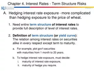
Chapter 4. Interest Rates - Term Structure Risks. A. Hedging interest rate exposure - more complicated than hedging exposure to the price of wheat . 1 . Need entire term structure of interest rates to provide full description of level of interest rates.

Chapter 4. Interest Rates - Term Structure Risks
E N D
Presentation Transcript
Chapter 4. Interest Rates - Term Structure Risks A. Hedging interest rate exposure-more complicated than hedging exposure to the price of wheat. 1. Need entire term structure of interest rates to provide full description of level of interest rates. 2. Definition of term structure (or yield curve): The relation among interest rates on securities alike in every respect except term to maturity. a. For example, plot gov't securities with maturities from 1 month to 20 years. b. To hedge interest rate exposure, must decide: i. maturity of interest rate exposure, ii. maturity of hedge you require.
B. Types of Rates. 1. Treasury Rates – paid on debt issued by government. Assume governments won’t default (can print money). Taxes & Regulations mean Treasury issues have artificial demand. Treasury Rates are not truly “riskfree” - they are too low. 2. LIBOR– London Interbank Offer Rate Rate that large international banks fund activities; Used as “riskfree rate.” Rate that one int’l bank lends / borrows at with another (default risk ≈ 0). 3. Repo Rate – rate on repurchase agreement. One institution needs short term cash, another has it; First institution deposits Treasury Securities with other, receives cash; Promises to repurchase securities in near future. Difference between cash received now & paid later determines repo rate. (default risk ≈ 0): If first defaults, second keeps Treasury Securities; If second defaults, first keeps cash. Popular vehicle for short term borrowing / lending.
C. Measuring Interest Rates Continuous Compounding & Discounting. 1. Amount A invested for n years at R per annum. a. compounded once/year, get A(1+R)n . b. compounded m times/year, get A(1+R/m)mn. c. Example: for n = 1 year, A = $100, R = 10%; m=1: get $100 x 1.10= $110. m=2: get $100 x 1.052= $110.25 ($5 x .10 x ½ year) m=4: get $100 x 1.0254= $110.38 m: get AeRn = $100e.10= $110.52 2. Continuous compounding, AeRn; eRn (1+R)n ; Continuous discounting, Ae-Rn; e-Rn1 / (1+R)n .
C. Measuring Interest Rates 3. Graphy Defn: e = lim(1 + 1/m)m │ex m │ e │ . . . . . │ . eR= lim(1 + R/m)m │ . m │ . │ . │ . Observe: ln(1)= 0; │ . │ . ln(x) ln(e)= 1;1 │ . . . . . . . . . . │ . . e0= 1; │ . . │ . . e1= e. │ . . │ . . __________________________│_____________________________________x │ 1e Discounting: ex< 1 if x < 0. │ │ Compounding: ex> 1 if x > 0. │ │ │
C. Measuring Interest Rates 4. Used to working with rates measured with annual, semiannual, or some other compounding frequency? Get used to continuous compounding / discounting! a. Can convert a continuously compounded rate to an equivalent rate compounded m times per annum: LetRc = interest rate with continuous compounding; Rm = equivalent rate compounded m times p.a. ThenAe(Rc)n = A(1 + Rm/ m)mn oreRc = (1 + Rm/ m)m This means: Rc = m ln(1 + Rm/ m) andRm = m ( eRc / m - 1) These equations convert a continuously compounded rate to an equivalent rate compounded m times p.a., & vice versa.
D. Zero Rates (or Spot Rates) 1. n-year Zero Rate: interest rate on n-year investmt. a. Assume no intermediate payments; all principle & interest paid after n years. b. Also called “n-year zero coupon rate.” 2. Zero Rates are determined by bootstrapping, using market prices on Treasury Securities with different maturities. Result is Zero-Coupon Yield Curve. See below and example in Hull.
E. Bond Pricing 1. Most bonds pay periodic coupons + face value at maturity. 2. Bond Price (PB= NPV of cash flows discounted at proper zero rates) Example: Face Value = F = $100; C / F = 6%; Coupon paid semi-annually, c = $3; Zero Rates: MaturityZero rate % (discount 0.55.0 rates) 1.05.8 1.56.4 2.06.8 PB = 3e-.05 x 0.5+ 3e-.058 x 1.0+ 3e-.064 x 1.5+ 103e-.068 x 2.0 = $98.39 At Discount; PB < F if y > C/F (6.76> 6). [At Premium; PB > F if y < C/F.] ($98.39 < $100)(Bond yield) 3. Bond Yield: single discount rate that equates cash flows to mkt value. Same Example: Let mkt value = PB = $98.39; Bond Yield (y) is solution to: $98.39 = 3e -y x 0.5+ 3e -y x 1.0+ 3e -y x 1.5+ 103e -y x 2.0 ; Here, y= 6.76%.
F. Bootstrapping Method to Determine Zero Rates Sample Data: Bond Time to Annual Bond Principal Maturity Coupon Price . $100 .25 $0 $97.5 $100 .50 $0 $94.9 $100 1.00 $0 $90.0 $100 1.50 $8$96.0 $100 2.00 $12 $101.6 1. An amount $2.5 can be earned on $97.5 during 3 months. • The 3-mo rate = Rm = 4 x ($2.5/$97.5) = 10.256%with qtrly compounding. • This is Rc = 10.127%with continuous compounding.(See formula for Rcon page 1-5.) 4. Similarly, the 6-month & 1-year rates = Rc = 10.469% & 10.536%, with continuouscompounding. 5. To calculate the 1.5-year rate, we solve the following : $96 = 4 e-.10469 x 0.5 + 4 e-.10536 x 1.0 + 104 e -Rcx 1.5 to get Rc= 0.10681 or 10.681%. 6. Similarly the two-year rate is computed to be 10.808%.
F. Bootstrapping Method Zero Rate Yield Curve Calculated from Example Zero Rate (%) 10.808 10.681 10.536 10.469 10.127 Maturity (years)
G. Forward Rates Rates implied by current spot rates for periods in the future. 1. Calculation of Forward Rates. (Assume all rates are continuously compounded.) Spot Rate for Forward Rate Year n-year investmtfor nth year (n) (% per annum) (% per annum). 1 10.0 -- 10.0% for 1yr $100e.10 = $110.52 in 1yr. 2 10.5 11.0-- 10.5% for 2yr $100e.105 x 2 = $123.37 in 2yr. 3 10.8 11.4 4 11.0 11.6 Forward rate for year 2 is rate implied by spot rates 5 11.1 11.5 . for future period between end of yr 1 & end of yr 2. 2. How do you get Forward rate for year 2 = r2 = 11.0? a. Suppose you have $100 available for 2 years. Two choices: i. Can invest 2 years at 2-yr spot rate (10.5); Will earn 100 e .105x 2 = $123.37 ii. Can invest 1 year at 1-yr spot rate (10.0), & reinvest yr2 at future 1-yr spot rate (r1,2 ); Will earn 100 e .10 e r1,2 = 100e(.10 + r1,2) b. Problem: Today don't know future 1-yr spot rate (r1,2). Forward rate for yr 2 (r2) is future 1-yr spot rate that would give same total result as i: 100 e (.10 + r2) = 100 e .105 x 2if (.10 + r2 ) = .105 x 2or r2 = .11 (Intuition: To get 10.5% for 2 years, must get 11% the 2nd year.)
G. Forward Rates Spot Rate for Forward Rate Year n-year investmt for nth year (n) (% per annum) (% per annum). 1 10.0 2 10.5 11.0 Forward rate for year 3 = r3 3 10.8 11.4 is rate implied by spot rates 4 11.0 11.6 for future period between 5 11.1 11.5 . end of year 2 & end of year 3. 3.How do you get r3? Suppose you have $ available for 3 years. Two choices: i. Can invest for 3 years at 3-yr spot rate (10.8); Will earn 100e .108 x 3 ii. Can invest for 2 years at 2-yr spot rate (10.5), & reinvest for yr 3 at future 1-yr spot rate (r1,3) ; Will earn 100 e .105 x 2e r1,3 = 100 e (.105 x 2 + r1,3) Forward rate for yr 3 (r3) is future1-yr spot rate that would give the same result as i. 100 e (.105 x 2 + r3) = 100e .108 x 3if .105 x 2 + r3 = .108 x 3or r3 = .114 (To get 10.8% for 3 years, must get 11.4% 3rd yr.) [ .21 + r3= .324 ] [ = .324 - .21]
G. Forward Rates Spot Rate for Forward Rate Year n-year investmtfor nth year (n) (% per annum) (% per annum). 1 10.0 2 10.5 11.0 General Formula: 3 10.8 11.4 Let r = spot rate for T years; 4 11.0 11.6 r* = spot rate for T* years; 5 11.1 11.5 . where T* > T. 4. General formula for the forward rate between periods T and T*: ╔═══════════════════╗ ║ r = (r*T* - rT) / (T* - T) ║ ╚═══════════════════╝ Example: 1-year forward rate for year 4 (r4 ); T = 3, T* = 4, r = .108, r* = .11, r4= (.11 x 4 - .108 x 3) / (4 - 3) = .44 - .324 = .116
G. Forward Rates 5. Assuming you can borrow or invest at any spot rate, you can lock in forward rate for borrowing or lending in any future period. Calculation of Forward Rates . Spot Rate for Forward Rate Year n-year investmtfor nth year (n) (% per annum) (% per annum). 1 10.0 2 10.5 11.0 3 10.8 11.4 4 11.011.6 5 11.1 11.5 . i. Borrow $100 @ 11% for 4 years; ii. Invest this money at 10.8% for 3 years; iii. Result: inflow at end of yr 3 = 100 e .108 x 3 = $138.26 outflow at end of yr 4 = 100 e .11 x 4 = $155.27 iv. Since 155.27 = 138.26 e .116 , money is being borrowed for the fourth year at 11.6%.
H. The Zero-Coupon Yield Curve 1.Defn: Relation between yields on zero-coupon bonds and maturity. Calculation of Forward Rates . yield Spot Rate for Forward Rate │ Year n-year investmtfor nth year │ (n) (% per annum) (% per annum). │ 1 10.0 │ 2 10.5 11.0 │ 3 10.8 11.4 │ 4 11.0 11.6 │ 5 11.1 11.5 . │________________________________ maturity 2.Forward Rate Yield Curve; relates forward rates to maturity. ** a. If yield curve is upward sloping, zero-coupon yield curve is belowforward rate yield curve. 3.Zero-Coupon Yield Curve versus Yield Curve for Coupon-Bearing Bonds. ** a. If yield curve is upward sloping, zero-coupon yield curve is above yield curve for coupon-bearing bonds. Yield on coupon-bearing bonds is affected by fact that investor gets some payments before maturity, when discount rates are lower than maturity rate. ** b. If yield curve is downward sloping, opposite. Forward curve Zero-coupon curve Coupon-bearing bond curve
I. Forward Rate Agreements (FRA’s) 1. OTC agreement that certain interest rate (RK) will apply to certain principal (L) during specified future period (T1 to T2). Can promise to lend / borrow with FRA. 2.Defns: L= principal; RK = FRA interest earned over T2 - T1 (agreed to in FRA); RF = forward LIBOR over T2 - T1 (expected borrowing cost); R = actual LIBOR over T2 - T1 (actual borrowing cost). Hull calls this RM. 3. Cash Flows for holding FRA (promise to lend in future): T1: +L ; borrow from bank later, at R; -L ; deposit according to FRA agreement. T2: +L [ 1 + RK ( T2 -T1 ) ] earned in FRA agreement; -L [ 1 + R ( T2 -T1 ) ] paid to bank. Will eventually get to keep: L (RK - R) (T2 - T1 ). Problem: Today we don’t know future borrowing rate, R; But we do know forward LIBOR, RF;Assume this isexpectedborrowing rate. Thus, today’s expectation of what we will get to keep: L (RK - RF ) (T2 - T1 ). 4.Value of FRA today= L (RK - RF) (T2 -T1) e-R2 T2; where R2 = T2 - pd zero spot rate. This is NPV of expected future cash flows; Value of promise to lend over T2 -T1.
J. Theories of the Term Structure 1.Expectations Theory: Long term spot rates reflect unbiased expectations of future short term spot rates; i.e., forward rates = expected future spot rates. Assumptions: i. Different maturities are perfect substitutes; ii. Money available for 2 years? – indifferent about investing 1 or 2 years … Implies: Shape of yield curve reveals expectations about whether rates will ↑ or ↓. i. If, market expects spot rates to remain stable. forward rates = spot rates, & yield curve is flat. ii. If market expects spot rates to rise in future, forward rates > spot rates, & yield curve slopes upward. iii. If market expects spot rates to fall, forward rates < spot rates, & yield curve slopes downward. iv. If market expects rates to first rise then fall, yield curve may have “bump."
J. Theories of the Term Structure 2.Liquidity Preference Theory: Investors prefer to invest short term, & will demand a premium for long positions. Borrowers prefer to borrow long term, & will pay a premium for long positions. Long term spot rates reflect expectations of future short term spot rates that are biased upward by a liquidity premium ; forward rates = expected future spot rates + liquidity premium. i. If market expects spot rates to remain stable, forward rates > spot rates by liquidity prem, & yield curve slightly upward sloping. ii. If market expects spot rates to rise, forward rates > spot rates by more than l.p., & yield curve is steeper than (i). iii. If market expects spot rates to fall, forward rates may be <, =, or > spot rates, depending on size of liquidity premium and how much mkt expects rates to fall. (Flatter than i., or slopes downward.) iv. 'Normal' yield curve is upward sloping; Downward sloping yield curve is rare.